Notebook

A Dockerfile that will produce a container with all the dependencies necessary to run this notebook is available here.

In [1]:

%matplotlib inline

In [2]:

from IPython.display import HTML

In [3]:

from edward.stats import bernoulli, normal, uniform
from edward.models import Normal
from matplotlib import pyplot as plt
from matplotlib.animation import ArtistAnimation
from matplotlib.patches import Ellipse
import numpy as np
import pandas as pd
import pymc3 as pm
from pymc3.distributions import draw_values
from pymc3.distributions.dist_math import bound
from pymc3.math import logsumexp
import scipy as sp
import seaborn as sns
import tensorflow as tf
from theano import shared, tensor as tt

In [4]:

# configure pyplot for readability when rendered as a slideshow and projected
plt.rc('figure', figsize=(8, 6))

LABELSIZE = 14
plt.rc('axes', labelsize=LABELSIZE)
plt.rc('axes', titlesize=LABELSIZE)
plt.rc('figure', titlesize=LABELSIZE)
plt.rc('legend', fontsize=LABELSIZE)
plt.rc('xtick', labelsize=LABELSIZE)
plt.rc('ytick', labelsize=LABELSIZE)

plt.rc('animation', writer='avconv')

In [5]:

blue, green, red, purple, gold, teal = sns.color_palette()

In [6]:

SEED = 69972 # from random.org, for reproducibility

np.random.seed(SEED)

Variational Inference in Python¶

PyData DC 2016¶

October 8, 2016¶

@AustinRochford — Monetate Labs ¶

arochford@monetate.com ¶

Bayesian Inference¶

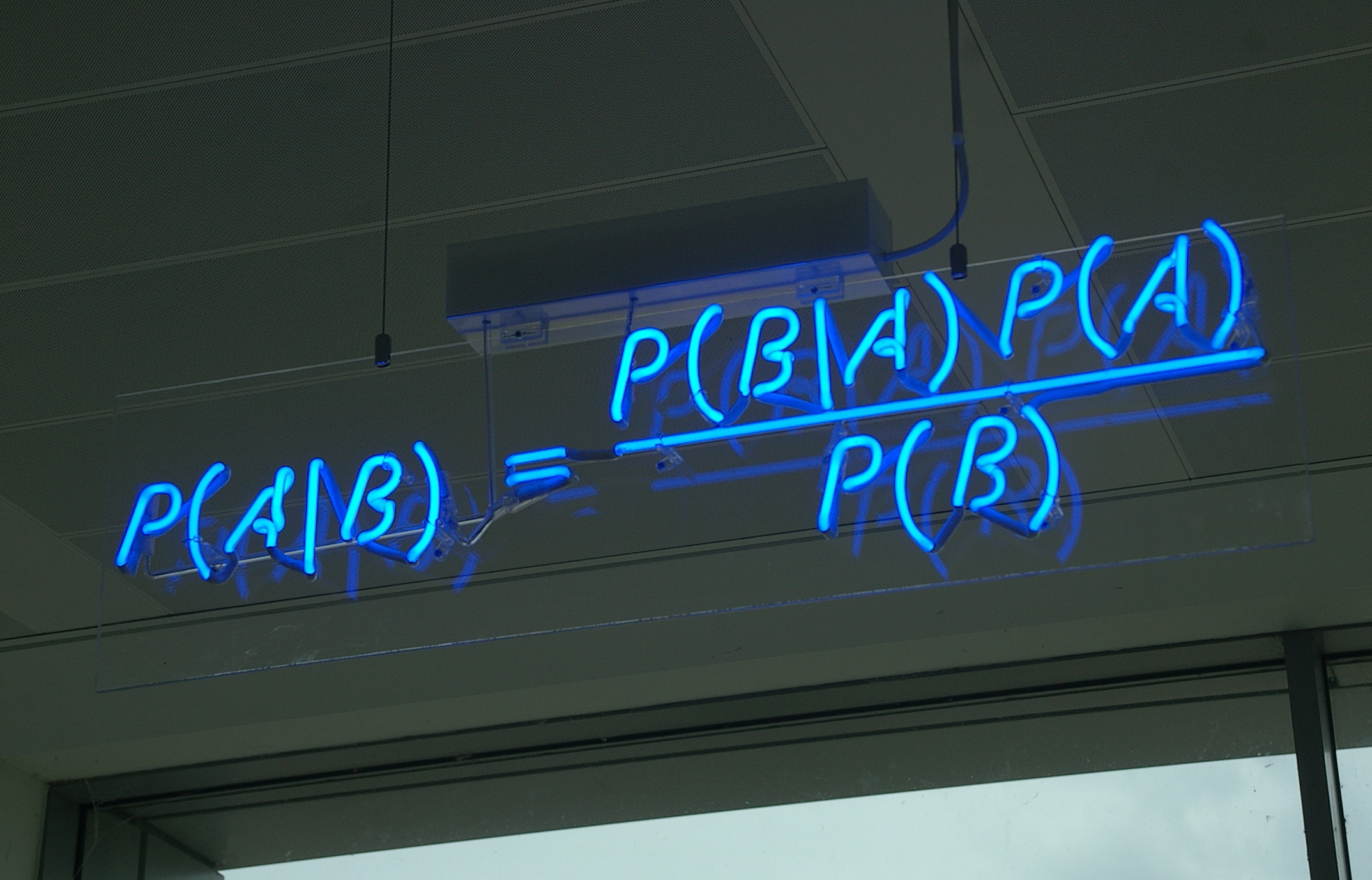
The posterior distribution is equal to the joint distribution divided by the marginal distribution of the evidence.

$\color{red}{P(\theta\ |\ \mathcal{D})} = \frac{\color{blue}{P(\mathcal{D}\ |\ \theta)\ P(\theta)}}{\color{green}{P(\mathcal{D})}} = \frac{\color{blue}{P(\mathcal{D}, \theta)}}{\color{green}{\int P(\mathcal{D}\ |\ \theta)\ P(\theta)\ d\theta}}$

For many useful models the marginal distribution of the evidence is hard or impossible to calculate analytically.

Modes of Bayesian Inference¶

Conjugate models with closed-form posteriors
Markov chain Monte Carlo algorithms
Approximate Bayesian computation
Distributional approximations
- Laplace approximations, INLA
- Variational inference

Markov Chain Monte Carlo Algorithms¶

Construct a Markov chain whose stationary distribution is the posterior distribution
Sample from the Markov chain for a long time
Approximate posterior quantities using the empirical distribution of the samples

To produce an interesting MCMC animation, we simulate a linear regression data set and animate samples from the posteriors of the regression coefficients.

In [7]:

x_animation = np.linspace(0, 1, 100)
y_animation = 1 - 2 * x_animation + np.random.normal(0., 0.25, size=100)

In [8]:

fig, ax = plt.subplots(figsize=(8, 6))

ax.scatter(x_animation, y_animation,
           c=blue);

ax.set_title('MCMC Animation Data Set');

In [9]:

with pm.Model() as mcmc_animation_model:
    intercept = pm.Normal('intercept', 0., 10.)
    slope = pm.Normal('slope', 0., 10.)
    
    tau = pm.Gamma('tau', 1., 1.)
    
    y_obs = pm.Normal('y_obs', intercept + slope * x_animation, tau=tau,
                      observed=y_animation)
    
    animation_trace = pm.sample(5000)

Applied log-transform to tau and added transformed tau_log_ to model.
Assigned NUTS to intercept
Assigned NUTS to slope
Assigned NUTS to tau_log_

WARNING (theano.tensor.blas): We did not found a dynamic library into the library_dir of the library we use for blas. If you use ATLAS, make sure to compile it with dynamics library.

 [-------100%-------] 5000 of 5000 in 3.3 sec. | SPS: 1521.7 | ETA: 0.0

In [10]:

animation_cov = np.cov(animation_trace['intercept'],
                       animation_trace['slope'])

animation_sigma, animation_U = np.linalg.eig(animation_cov)
animation_angle = 180. / np.pi * np.arccos(np.abs(animation_U[0, 0]))

In [11]:

animation_fig = plt.figure()

e = Ellipse((animation_trace['intercept'].mean(), animation_trace['slope'].mean()),
            2 * np.sqrt(5.991 * animation_sigma[0]), 2 * np.sqrt(5.991 * animation_sigma[1]),
            angle=animation_angle, zorder=5)
e.set_alpha(0.5)
e.set_facecolor(blue)
e.set_zorder(9);

animation_images = [(plt.plot(animation_trace['intercept'][-(iter_ + 1):],
                              animation_trace['slope'][-(iter_ + 1):],
                              '-o', c='k', alpha=0.5, zorder=10)[0],)
                    for iter_ in range(50)]

animation_ax = animation_fig.gca()
animation_ax.add_artist(e);

animation_ax.set_xticklabels([]);
animation_ax.set_xlim(0.75, 1.3);

animation_ax.set_yticklabels([]);
animation_ax.set_ylim(-2.5, -1.5);

mcmc_animation = ArtistAnimation(animation_fig, animation_images,
                                 interval=100, repeat_delay=5000,
                                 blit=True)
mcmc_video = mcmc_animation.to_html5_video()

In [12]:

HTML(mcmc_video)

Out[12]:

Beta-Binomial Model¶

We observe three successes in ten trials, and want to infer the true success probability.

In [13]:

x_beta_binomial = np.array([1, 1, 1, 0, 0, 0, 0, 0, 0, 0])

$p \sim U(0, 1)$

In [14]:

import pymc3 as pm

with pm.Model() as beta_binomial_model:
    p_beta_binomial = pm.Uniform('p', 0., 1.)

Applied interval-transform to p and added transformed p_interval_ to model.

$\begin{align*} P(X_i = 1\ |\ p) & = p \end{align*}$

In [15]:

with beta_binomial_model:
    x_obs = pm.Bernoulli('y', p_beta_binomial,
                         observed=x_beta_binomial)

$p\ \left|\ \sum_{i = 1}^{10} X_i \right. = 3 \sim \textrm{Beta}(4, 8)$

In [16]:

# plot the true beta-binomial posterior distribution
fig, ax = plt.subplots()

prior = sp.stats.uniform(0, 1)
posterior = sp.stats.beta(1 + x_beta_binomial.sum(), 1 + (1 - x_beta_binomial).sum())

plot_x = np.linspace(0, 1, 100)
ax.plot(plot_x, prior.pdf(plot_x),
        '--', c='k', label='Prior');

ax.plot(plot_x, posterior.pdf(plot_x),
        c=blue, label='Posterior');

ax.set_xticks(np.linspace(0, 1, 5));
ax.set_xlabel(r'$p$');

ax.set_yticklabels([]);

ax.legend(loc=1);

In [17]:

fig

Out[17]:

In [18]:

BETA_BINOMIAL_SAMPLES = 50000
BETA_BINOMIAL_BURN = 10000
BETA_BINOMIAL_THIN = 20

In [19]:

with beta_binomial_model:
    beta_binomial_trace_ = pm.sample(BETA_BINOMIAL_SAMPLES, random_seed=SEED)

beta_binomial_trace = beta_binomial_trace_[BETA_BINOMIAL_BURN::BETA_BINOMIAL_THIN]

Assigned NUTS to p_interval_
 [-------100%-------] 50000 of 50000 in 13.1 sec. | SPS: 3829.8 | ETA: 0.0

In [20]:

bins = np.linspace(0, 1, 50)
ax.hist(beta_binomial_trace['p'], bins=bins, normed=True,
        color=green, lw=0., alpha=0.5,
        label='MCMC approximate posterior');

ax.legend();

In [21]:

fig

Out[21]:

Pros¶

Asymptotically unbiased: converges to the true posterior afer many samples
Model-agnostic algorithms
Well-studied for more than 60 years

Cons¶

Can take a long time to converge
- Can be difficult to assess convergence
Difficult to scale

Variational Inference¶

Choose a class of approximating distributions
Find the best approximation to the true posterior

Variational inference minimizes the Kullback-Leibler divergence

$\mathbb{KL}(\color{purple}{q(\theta)} \parallel \color{red}{p(\theta\ |\ \mathcal{D})}) = \mathbb{E}_q\left(\log\left(\frac{\color{purple}{q(\theta)}}{\color{red}{p(\theta\ |\ \mathcal{D})}}\right)\right)$

from approximate distributons, but we can't calculate the true posterior distribution.

Minimizing the Kullback-Leibler divergence

$\mathbb{KL}(\color{purple}{q(\theta)} \parallel \color{red}{p(\theta\ |\ \mathcal{D})}) = -(\underbrace{\mathbb{E}_q(\log \color{blue}{p(\mathcal{D}, \theta))} - \mathbb{E}_q(\color{purple}{\log q(\theta)})}_{\color{orange}{\textrm{ELBO}}}) + \log \color{green}{p(\mathcal{D})}$

is equivalent to maximizing the Evidence Lower BOund (ELBO), which only requires calculating the joint distribution.

Variational Inference Example¶

In this example, we minimize the Kullback-Leibler divergence between a full-rank covariance Gaussian distribution and a diagonal covariance Gaussian distribution.

In [22]:

SIGMA_X = 1.
SIGMA_Y = np.sqrt(0.5)
CORR_COEF = 0.75

true_cov = np.array([[SIGMA_X**2, CORR_COEF * SIGMA_X * SIGMA_Y],
                     [CORR_COEF * SIGMA_X * SIGMA_Y, SIGMA_Y**2]])
true_precision = np.linalg.inv(true_cov)

approx_sigma_x, approx_sigma_y = 1. / np.sqrt(np.diag(true_precision))

In [23]:

fig, ax  = plt.subplots(figsize=(8, 8))
ax.set_aspect('equal');


var, U = np.linalg.eig(true_cov)
angle = 180. / np.pi * np.arccos(np.abs(U[0, 0]))

e = Ellipse(np.zeros(2), 2 * np.sqrt(5.991 * var[0]), 2 * np.sqrt(5.991 * var[1]), angle=angle)
e.set_alpha(0.5)
e.set_facecolor(blue)
e.set_zorder(10);
ax.add_artist(e);

ax.set_xlim(-3, 3);
ax.set_xticklabels([]);

ax.set_ylim(-3, 3);
ax.set_yticklabels([]);

rect = plt.Rectangle((0, 0), 1, 1, fc=blue, alpha=0.5)
ax.legend([rect],
          ['True distribution'],
          bbox_to_anchor=(1.5, 1.));

In [24]:

fig

Out[24]:

Approximate the true distribution using a diagonal covariance Gaussian from the class

$\mathcal{Q} = \left\{\left.N\left(\begin{pmatrix} \mu_x \\ \mu_y \end{pmatrix}, \begin{pmatrix} \sigma_x^2 & 0 \\ 0 & \sigma_y^2\end{pmatrix}\ \right|\ \mu_x, \mu_y \in \mathbb{R}^2, \sigma_x, \sigma_y > 0\right)\right\}$

In [25]:

vi_e = Ellipse(np.zeros(2), 2 * np.sqrt(5.991) * approx_sigma_x, 2 * np.sqrt(5.991) * approx_sigma_y)
vi_e.set_alpha(0.4)
vi_e.set_facecolor(red)
vi_e.set_zorder(11);
ax.add_artist(vi_e);

vi_rect = plt.Rectangle((0, 0), 1, 1, fc=red, alpha=0.75)

ax.legend([rect, vi_rect],
          ['Posterior distribution',
           'Variational approximation'],
          bbox_to_anchor=(1.55, 1.));

In [26]:

fig

Out[26]:

Pros¶

A principled method to trade complexity for bias
Optimization theory is applicable
- Assesment of convergence
- Scalability

Cons¶

Biased estimate of the true posterior
- Better for prediction than interpretation
Model-specific algorithms

Mean field variational inference¶

Assume the variational distribution factors independently as $q(\theta_1, \ldots, \theta_n) = q(\theta_1) \cdots q(\theta_n)$

The variational approximation can be found by coordinate ascent

$\begin{align*} q(\theta_i) & \propto \exp\left(\mathbb{E}_{q_{-i}}(\log(\mathcal{D}, \boldsymbol{\theta}))\right) \\ q_{-i}(\boldsymbol{\theta}) & = q(\theta_1) \cdots q(\theta_{i - 1})\ q(\theta_{i + 1}) \cdots q(\theta_n) \end{align*}$

Coordinate Ascent Cons¶

Calculations are tedious, even when possible
Convergence is slow when the number of parameters is large

Automating Variational Inference in Python¶

Maximize ELBO using gradient ascent instead of coordinate ascent
Tensor libraries calculate ELBO gradients automatically

Python Package	Tensor Library	Variational Inference Algorithm(s)
Edward	TensorFlow	Black Box Variational Inference (BBVI)
PyMC3	Theano	Automatic Differentiation Variational Inference (ADVI)

Common themes¶

Monte Carlo estimate of the ELBO gradient
Minibatch estimates of the joint distribution

BBVI and ADVI arise from different ways of calculating the ELBO gradient

Mathematical details¶

Monte Carlo estimate of the ELBO gradient
- For samples $\tilde{\theta}_1, \ldots, \tilde{\theta}_K \sim q(\theta)$
Minibatch estimate of joint distribution
- Sample data points $\mathbf{x}_1, \ldots, \mathbf{x}_B$ from $\mathcal{D}$

BBVI and ADVI arise from different ways of calculating $\nabla \left(\log p(\mathcal{D}, \cdot) - \log q(\cdot)\right)$

Variational Inference with Edward¶

Black Box Variational Inference (BBVI)¶

Model-agnostic
- Requires the ability to compute the joint distribution
- Required the ability to differentiate the variational distribution

Mathematical details¶

For samples $\tilde{\theta}_1, \ldots, \tilde{\theta}_K \sim q(\theta)$

$\begin{align*} \nabla \textrm{ELBO} & = \mathbb{E}_q \left(\nabla\left(\log p(\mathcal{D}, \theta) - \log q(\theta)\right)\right) \\ & = \mathbb{E}_q \left(\left(\log p(\mathcal{D}, \theta) - \log q(\theta)\right) \nabla \log q(\theta)\right) \\ & \approx \frac{1}{K} \sum_{i = 1}^K \left(\log p(\mathcal{D}, \tilde{\theta}_i) - \log q(\tilde{\theta}_i)\right) \nabla \log q(\tilde{\theta}_i) \end{align*}$

Beta-binomial model¶

In [27]:

import edward as ed
from edward.models import Bernoulli, Beta, Uniform

ed.set_seed(SEED)

# probability model
p = Uniform(a=0., b=1.)
x_edward_beta_binomial = Bernoulli(p=p)

data = {x_edward_beta_binomial: x_beta_binomial}

In [28]:

def tf_variable(shape=None):
    """
    Create a TensorFlow Variable with the given shape
    """
    shape = shape if shape is not None else []
    
    return tf.Variable(tf.random_normal(shape))

def tf_positive_variable(shape=None):
    """
    Create a TensorFlow Variable that is constrained to be positive
    with the given shape
    """
    return tf.nn.softplus(tf_variable(shape))

In [29]:

# variational approximation
q_p = Beta(a=tf_positive_variable(),
           b=tf_positive_variable())
q = {p: q_p}

In [30]:

%%time
beta_binomial_inference = ed.MFVI(q, data)
beta_binomial_inference.run(n_iter=10000, n_print=None)

CPU times: user 5.83 s, sys: 880 ms, total: 6.71 s
Wall time: 4.63 s

In [31]:

# plot edward's approximation to the true beta-binomial posterior
fig, ax = plt.subplots()

ed_posterior = sp.stats.beta(beta_binomial_inference.latent_vars[p].distribution.a.eval(),
                             beta_binomial_inference.latent_vars[p].distribution.b.eval())

plot_x = np.linspace(0, 1, 100)
ax.plot(plot_x, prior.pdf(plot_x),
        '--', c='k', label='Prior');

ax.plot(plot_x, posterior.pdf(plot_x),
        c=blue, label='Posterior');
ax.plot(plot_x, ed_posterior.pdf(plot_x),
        c=red, label='Edward posterior');


ax.set_xticks(np.linspace(0, 1, 5));
ax.set_xlabel(r'$p$');

ax.set_yticklabels([]);

ax.legend(loc=1);

In [32]:

fig

Out[32]:

In [33]:

from edward.models import PyMC3Model

# probability model
x_beta_binomial_obs = shared(np.zeros(1))

with pm.Model() as beta_binomial_model_untransformed:
    p = pm.Uniform('p', 0., 1., transform=None)
    x_beta_binomial_ = pm.Bernoulli('x', p, observed=x_beta_binomial_obs)
    
pymc3_data = {x_beta_binomial_obs: x_beta_binomial}
pymc3_beta_binomial_model = PyMC3Model(beta_binomial_model_untransformed)

In [34]:

%%time
# variational distribution
pymc3_q_p = Beta(a=tf_positive_variable(),
                 b=tf_positive_variable())
pymc3_q = {'p': pymc3_q_p}

pymc3_beta_binomial_inference = ed.MFVI(pymc3_q, pymc3_data,
                                        pymc3_beta_binomial_model)
pymc3_beta_binomial_inference.run(n_iter=30000, n_print=None)

CPU times: user 29.3 s, sys: 5.54 s, total: 34.8 s
Wall time: 22.4 s

In [35]:

# plot a comparison of the variational approximations calculating using
# using the tensorflow and pymc3 models
fig, (tf_ax, pymc3_ax) = plt.subplots(ncols=2, sharex=True, sharey=True, figsize=(16, 6))

tf_ax.plot(plot_x, prior.pdf(plot_x),
           '--', c='k', label='Prior');

tf_ax.plot(plot_x, posterior.pdf(plot_x),
           c=blue, label='Posterior');
tf_ax.plot(plot_x, ed_posterior.pdf(plot_x),
           c=red, label='Edward posterior');


tf_ax.set_xticks(np.linspace(0, 1, 5));
tf_ax.set_xlabel(r'$p$');

tf_ax.set_yticklabels([]);

tf_ax.legend(loc=1);
tf_ax.set_title('TensorFlow Model');

pymc3_posterior = sp.stats.beta(pymc3_beta_binomial_inference.latent_vars['p'].distribution.a.eval(),
                                pymc3_beta_binomial_inference.latent_vars['p'].distribution.b.eval())

pymc3_ax.plot(plot_x, prior.pdf(plot_x),
              '--', c='k', label='Prior');

pymc3_ax.plot(plot_x, posterior.pdf(plot_x),
              c=blue, label='Posterior');
pymc3_ax.plot(plot_x, pymc3_posterior.pdf(plot_x),
              c=red, label='Edward posterior');


pymc3_ax.set_xticks(np.linspace(0, 1, 5));
pymc3_ax.set_xlabel(r'$p$');

pymc3_ax.set_yticklabels([]);
pymc3_ax.set_title('PyMC3 Model');

fig.suptitle('Beta-Binomial Mean Field Variational Inference with Edward');

In [36]:

fig

Out[36]:

Edward-supported modeling "languages"¶

Joint Distribution	Variational Distribution
TensorFlow Distributions	TensorFlow
PyMC3
Stan
Direction density calculations TensorFlow Numpy Pure Python

Congressional Ideal Points¶

The congressional ideal point model uses the 1984 congressional voting records data set from the UCI Machine Learning Repository.

In [37]:

%%bash
# download the data set, if we have not already
if [ ! -e /tmp/house-votes-84.data ]
then
    wget -O /tmp/house-votes-84.data \
        http://archive.ics.uci.edu/ml/machine-learning-databases/voting-records/house-votes-84.data
fi

Load and code the congressional voting data.

"No" votes ('n') are coded as zero, "yes" ('y') votes are coded as one, and skipped/unknown votes ('?') are coded as np.nan. The skipped/unknown votes will be dropped later.

Also, code the representative's parties.

In [38]:

N_BILLS = 16

vote_df = pd.read_csv('/tmp/house-votes-84.data',
                      names=['party'] + list(range(N_BILLS)))

vote_df.index.name = 'rep'

vote_df[vote_df == 'n'] = 0
vote_df[vote_df == 'y'] = 1
vote_df[vote_df == '?'] = np.nan

vote_df.party, parties = vote_df.party.factorize()
republican = (parties == 'republican').argmax()

n_reps = vote_df.shape[0]

Republicans ('republican') are coded as zero and democrats ('democrat') are coded as one.

In [39]:

parties

Out[39]:

Index(['republican', 'democrat'], dtype='object')

In [40]:

vote_df.head()

Out[40]:

	party	0	1	2	3	4	5	6	7	8	9	10	11	12	13	14	15
rep
0	0	0	1	0	1	1	1	0	0	0	1	NaN	1	1	1	0	1
1	0	0	1	0	1	1	1	0	0	0	0	0	1	1	1	0	NaN
2	1	NaN	1	1	NaN	1	1	0	0	0	0	1	0	1	1	0	0
3	1	0	1	1	0	NaN	1	0	0	0	0	1	0	1	0	0	1
4	1	1	1	1	0	1	1	0	0	0	0	1	NaN	1	1	1	1

Transform the voting data from wide form to "tidy" form; that is, one row per representative and bill combination.

If you haven't already, go read Hadley Wickham's Tidy Data paper.

In [41]:

long_vote_df = (pd.melt(vote_df.reset_index(),
                        id_vars=['rep', 'party'], value_vars=list(range(N_BILLS)),
                        var_name='bill', value_name='vote')
                  .dropna()
                  .astype(np.int64))

In [42]:

grid = sns.factorplot('bill', 'vote', 'party', long_vote_df,
                      kind='bar', ci=None, size=8, aspect=1.5, legend=False,
                      palette=[red, blue]);
grid.set_axis_labels('Bill', 'Percent of party\'s\nrepresentatives voting for bill');
grid.add_legend(legend_data={parties[int(key)].capitalize(): artist
                             for key, artist in grid._legend_data.items()});
grid.fig.suptitle('Key 1984 Congressional Votes');

In [43]:

grid.fig

Out[43]:

Idea:

Representatives (αi) and bills (βj) each have an ideal point on a spectrum of conservativity
- If a representative's and bill's ideal points are the same, the representative has a 50% chance of voting for the bill

Bills also have an ability to discriminate (γj) between conservative and liberal representatives
- Some bills have broad bipartisan support, while some provoke votes along party lines

Representative ideal points¶

$\begin{align*} \color{blue}{\alpha_1}, \ldots, \color{blue}{\alpha_N} & \sim N(0, 1) \end{align*}$

In [44]:

def normal_log_prior(value, loc=0., scale=1.):
    return tf.reduce_sum(normal.log_pdf(value, loc, scale))

Bill ideal points and discriminative abilities¶

$\begin{align*} \mu_{\beta} & \sim N(0, 1) \\ \sigma_{\beta} & \sim U(0, 1) \\ \color{green}{\beta_1}, \ldots, \color{green}{\beta_K} & \sim N(\mu_{\beta}, \sigma_{\beta}^2) \end{align*}$

$\begin{align*} \mu_{\gamma} & \sim N(0, 1) \\ \sigma_{\gamma} & \sim U(0, 1) \\ \color{red}{\gamma_1}, \ldots, \color{red}{\gamma_K} & \sim N(\mu_{\gamma}, \sigma_{\gamma}^2) \end{align*}$

In [45]:

def hierarchical_log_prior(value, mu, sigma):
    log_hyperprior = normal_log_prior(mu) + uniform.log_pdf(sigma, 0., 1.)

    return log_hyperprior + normal_log_prior(value, loc=mu, scale=sigma)

In [46]:

def log_prior(alpha,
              beta, mu_beta, sigma_beta,
              gamma, mu_gamma, sigma_gamma):
    """
    Combine the log priors for alpha, beta, and gamma into the
    overall prior
    """
    return normal_log_prior(alpha) \
            + hierarchical_log_prior(beta, mu_beta, sigma_beta) \
            + hierarchical_log_prior(gamma, mu_gamma, sigma_gamma)

Note that we do not specify a hierarchical prior on $\alpha_1, \ldots, \alpha_K$ in order to ensure that the model is identifiable. See Practical issues in implementing and understanding Bayesian ideal point estimation for an in-depth discussion of identification issues in Bayesian ideal point models.

Observation model¶

$\begin{align*} \mathbb{P}(\textrm{Representative }i \textrm{ votes for bill }j\ |\ \color{blue}{\alpha_i}, \color{green}{\beta_j}, \color{red}{\gamma_j}) & = \frac{1}{1 + \exp(-\color{red}{\gamma_j} \left(\color{blue}{\alpha_i} - \color{green}{\beta_j}\right))} \end{align*}$

In [47]:

def long_from_indices(short, indices):
    return tf.gather(short, tf.cast(indices, tf.int64))

In [48]:

def log_like(vote, rep, bill, alpha, beta, gamma):
    # alpha, beta, and gamma have one entry for representative/bill,
    # index them to have one entry per representative/bill combination
    alpha_long = long_from_indices(alpha, rep)
    beta_long = long_from_indices(beta, bill)
    gamma_long = long_from_indices(gamma, bill)

    p = tf.sigmoid(gamma_long * (alpha_long - beta_long))

    return tf.reduce_sum(bernoulli.logpmf(vote, p))

Edward model¶

In [49]:

class IdealPoint:
    def log_prob(self, xs, zs):
        """
        xs is a dictionary of observed data
        zs is a dictionary of parameters
        
        Calculates the model's log joint distribution
        """
        # parameters
        alpha, beta, gamma = zs['alpha'], zs['beta'], zs['gamma']
        mu_beta, mu_gamma = zs['mu_beta'], zs['mu_gamma']
        sigma_beta, sigma_gamma = zs['sigma_beta'], zs['sigma_gamma']
        
        # observed data
        vote, bill, rep = xs['vote'], xs['bill'], xs['rep']

        # log joint distribution
        log_prior_ = log_prior(alpha,
                               beta, mu_beta, sigma_beta,
                               gamma, mu_gamma, sigma_gamma)
        log_like_ = log_like(vote, rep, bill,
                             alpha, beta, gamma)
        
        return log_prior_ + log_like_

ideal_point_model = IdealPoint()

In [50]:

ideal_point_data = {
    'vote': long_vote_df.vote.values,
    'bill': long_vote_df.bill.values,
    'rep': long_vote_df.rep.values
}

In [51]:

def tf_normal(shape=None):
    """
    Create a TensorFlow normal distribution with the given shape
    """
    return Normal(mu=tf_variable(shape),
                  sigma=tf_positive_variable(shape))

def tf_uniform(shape=None):
    """
    Create a TensorFlow uniform distribution with the given shape
    """
    a = tf_positive_variable(shape)
    
    return Uniform(a=a,
                   b=a + tf_positive_variable(shape))

BBVI inference¶

In [52]:

# variational distribution
q_alpha = tf_normal((n_reps,))

q_mu_beta = tf_normal()
q_sigma_beta = tf_uniform()
q_beta = tf_normal((N_BILLS,))

q_mu_gamma = tf_normal()
q_sigma_gamma = tf_uniform()
q_gamma = tf_normal((N_BILLS,))

q = {
    'alpha': q_alpha,
    'beta': q_beta, 'mu_beta': q_mu_beta, 'sigma_beta': q_sigma_beta,
    'gamma': q_gamma, 'mu_gamma': q_mu_gamma, 'sigma_gamma': q_sigma_gamma,
}

In [53]:

%%time
inference = ed.MFVI(q, ideal_point_data, ideal_point_model)
inference.run(n_iter=20000, n_print=None)

CPU times: user 1min 33s, sys: 30.2 s, total: 2min 4s
Wall time: 52.8 s

In [54]:

ideal_point_alpha_mean = inference.latent_vars['alpha'].mean().eval()
ideal_point_alpha_std = inference.latent_vars['alpha'].std().eval()

N_IDEAL_POINT_SAMPLES = 10000

ideal_point_alpha_samples = np.random.normal(ideal_point_alpha_mean[:, np.newaxis],
                                             ideal_point_alpha_std[:, np.newaxis],
                                             size=(n_reps, N_IDEAL_POINT_SAMPLES))

In [55]:

fig, ax = plt.subplots()

bins = np.linspace(-3, 3, 100)

is_republican = (vote_df.party == republican).values
ax.hist(ideal_point_alpha_samples[~is_republican].ravel(), bins=bins,
        color=blue, alpha=0.5, lw=0,
        label='Democrat');
ax.hist(ideal_point_alpha_samples[is_republican].ravel(), bins=bins,
        color=red, alpha=0.5, lw=0,
        label='Republican',);

ax.set_xlabel('Conservativity');
ax.set_yticklabels([]);

ax.legend(loc=1);
ax.set_title('Posterior Ideal Points');

In [56]:

fig

Out[56]:

Fun project: Recreate the Martin-Quinn dynamic ideal point model for ideology of U.S. Supreme Court justices with Edward

Variational Inference with PyMC3¶

Automatic Differentiation Variational Inference (ADVI)¶

Only applicable to differentiable probability models
Transform constrained parameters to be unconstrained
Approximate the posterior for unconstrained parameters with mean field Gaussian

Beta-binomial model¶

In [57]:

# plot the transformed (unconstrained) parameters
fig, (const_ax, trans_ax) = plt.subplots(ncols=2, figsize=(16, 6))

prior = sp.stats.uniform(0, 1)
posterior = sp.stats.beta(1 + x_beta_binomial.sum(),
                          1 + (1 - x_beta_binomial).sum())

# constrained distribution plots
const_x = np.linspace(0, 1, 100)
const_ax.plot(const_x, prior.pdf(const_x),
              '--', c='k', label='Prior');

def logit_trans_pdf(pdf, x):
    x_logit = sp.special.logit(x)
    return pdf(x_logit) / (x * (1 - x))

const_ax.plot(const_x, posterior.pdf(const_x),
              c=blue, label='Posterior');

const_ax.set_xticks(np.linspace(0, 1, 5));
const_ax.set_xlabel(r'$p$');
const_ax.set_yticklabels([]);
const_ax.set_title('Constrained Parameter Space');
const_ax.legend(loc=1);

# unconstrained distribution plots
def expit_trans_pdf(pdf, x):
    x_expit = sp.special.expit(x)
    return pdf(x_expit) * x_expit * (1 - x_expit)

trans_x = np.linspace(-5, 5, 100)
trans_ax.plot(trans_x, expit_trans_pdf(prior.pdf, trans_x),
              '--', c='k');
trans_ax.plot(trans_x, expit_trans_pdf(posterior.pdf, trans_x),
              c=blue);

trans_ax.set_xlim(trans_x.min(), trans_x.max());
trans_ax.set_xlabel(r'$\log\left(\frac{p}{1 - p}\right)$');
trans_ax.set_yticklabels([]);
trans_ax.set_title('Unconstrained Parameter Space');

Transformed distributions¶

In [58]:

fig

Out[58]:

In [59]:

%%time
with beta_binomial_model:
    advi_fit = pm.advi(n=20000, random_seed=SEED)

Iteration 0 [0%]: ELBO = -10.91
Iteration 2000 [10%]: Average ELBO = -7.76
Iteration 4000 [20%]: Average ELBO = -7.37
Iteration 6000 [30%]: Average ELBO = -7.24
Iteration 8000 [40%]: Average ELBO = -7.22
Iteration 10000 [50%]: Average ELBO = -7.17
Iteration 12000 [60%]: Average ELBO = -7.15
Iteration 14000 [70%]: Average ELBO = -7.19
Iteration 16000 [80%]: Average ELBO = -7.18
Iteration 18000 [90%]: Average ELBO = -7.19
Finished [100%]: Average ELBO = -7.2
CPU times: user 3.12 s, sys: 0 ns, total: 3.12 s
Wall time: 3.1 s

In [60]:

advi_bb_mu = advi_fit.means['p_interval_']
advi_bb_std = advi_fit.stds['p_interval_']
advi_bb_dist = sp.stats.norm(advi_bb_mu, advi_bb_std)

In [61]:

# plot the ADVI gaussian approximation to the unconstrained posterior
trans_ax.plot(trans_x, advi_bb_dist.pdf(trans_x),
              c=red, label='Variational approximation');

ADVI approxiation to transformed posterior¶

In [62]:

fig

Out[62]:

In [63]:

# plot the ADVI approximation to the true posterior
const_ax.plot(const_x, logit_trans_pdf(advi_bb_dist.pdf, const_x),
              c=red, label='Variational approximation');

ADVI approximation to posterior¶

In [64]:

fig

Out[64]:

Dependent Density Regression¶

The depdendent density regression uses LIDAR data from Larry Wasserman's book All of Nonparametric Statistics.

In [65]:

%%bash
# download the LIDAR data file, it is not already present
if [ ! -e /tmp/lidar.dat ]
then
    wget -O /tmp/lidar.dat http://www.stat.cmu.edu/~larry/all-of-nonpar/=data/lidar.dat
fi

In [66]:

# read and standardize the LIDAR data
lidar_df = (pd.read_csv('/tmp/lidar.dat',
                        sep=' *', engine='python')
              .assign(std_range=lambda df: (df.range - df.range.mean()) / df.range.std(),
                      std_logratio=lambda df: (df.logratio - df.logratio.mean()) / df.logratio.std()))

In [67]:

# plot the LIDAR dataset
fig, ax = plt.subplots()

ax.scatter(lidar_df.std_range, lidar_df.std_logratio,
           c=blue, zorder=10);

ax.set_xticklabels([]);
ax.set_xlabel('Range');

ax.set_yticklabels([]);
ax.set_ylabel('Log ratio');

ax.set_title('LIDAR Data');

In [68]:

fig

Out[68]:

Idea: A mixture of linear models, where the unknown number of mixture weights depend on $x$

In [69]:

# fit and plot a few linear models on different intervals
# of the LIDAR data
LIDAR_KNOTS = np.array([-1.75, 0., 0.5, 1.75])

for left_knot, right_knot in zip(LIDAR_KNOTS[:-1], LIDAR_KNOTS[1:]):
    between_knots = lidar_df.std_range.between(left_knot, right_knot)
    slope, intercept, *_ = sp.stats.linregress(lidar_df.std_range[between_knots].values,
                                               lidar_df.std_logratio[between_knots].values)

    knot_plot_x = np.linspace(left_knot - 0.25, right_knot + 0.25, 100)
    ax.plot(knot_plot_x, intercept + slope * knot_plot_x, 
            c=red, lw=2, zorder=100);
    
ax.set_xlim(-2.1, 2.1);

In [70]:

fig

Out[70]:

Mixture weights¶

The model has infinitely many mixture components, we truncate to $K$

$\begin{align*} \alpha_1, \ldots, \alpha_K & \sim N(0, 1) \\ \beta_1, \ldots, \beta_K & \sim N(0, 1) \\ \boldsymbol{\pi} \ |\ \boldsymbol{\alpha}, \boldsymbol{\beta}, x & \sim \textrm{Logit-Stick-Breaking}(\boldsymbol{\alpha} + \boldsymbol{\beta} x) \\ \end{align*}$

In [71]:

# turn the LIDAR observations into column vectors
# this is important for broadcasting in following
# calculations
std_range = lidar_df.std_range.values[:, np.newaxis]
std_logratio = lidar_df.std_logratio.values[:, np.newaxis]

The stick-breaking process transforms an arbitrary set of values in the interval $[0, 1]$ to a set of weights in $[0, 1]$ that sum to one.

In [72]:

def stick_breaking(v):
    """
    Perform a stick breaking transformation along
    the second axis of v
    """
    return v * tt.concatenate([tt.ones_like(v[:, :1]),
                               tt.extra_ops.cumprod(1 - v, axis=1)[:, :-1]],
                              axis=1)

In [73]:

K = 20

x_lidar = shared(std_range, broadcastable=(False, True))

with pm.Model() as lidar_model:
    alpha = pm.Normal('alpha', 0., 1., shape=K)
    beta = pm.Normal('beta', 0., 1., shape=K)
    
    v = tt.nnet.sigmoid(alpha + beta * x_lidar)
    pi = pm.Deterministic('pi', stick_breaking(v))

Component linear models¶

$\begin{align*} \gamma_1, \ldots, \gamma_K & \sim N(0, 100) \\ \delta_1, \ldots, \delta_K & \sim N(0, 100) \\ \tau_1, \ldots, \tau_K & \sim \textrm{Gamma}(1, 1) \\ Y_i\ |\ \gamma_i, \delta_i, \tau_i, x & \sim N(\gamma_i + \delta_i x, \tau_i^{-1}) \end{align*}$

In [74]:

with lidar_model:
    gamma = pm.Normal('gamma', 0., 100., shape=K)
    delta = pm.Normal('delta', 0., 100., shape=K)
    tau = pm.Gamma('tau', 1., 1., shape=K)

    ys = pm.Deterministic('ys', gamma + delta * x_lidar)

Applied log-transform to tau and added transformed tau_log_ to model.

Observation model¶

$\begin{align*} Y\ |\ \boldsymbol{\alpha}, \boldsymbol{\beta}, \boldsymbol{\gamma}, \boldsymbol{\delta}, \boldsymbol{\tau}, x & = \sum_{i = 1}^K \pi_i Y_i \\ \end{align*}$

The NormalMixture class is a bit of a hack to marginalize over the categorical indicators that would otherwise be necessary to implement a normal mixture model in PyMC3. This also speeds convergence in both MCMC and variational inference algorithms. See the Stan User's Guide and Reference Manual for more information on the benefits of marginalization.

In [75]:

def normal_mixture_rvs(*args, **kwargs):
    w = kwargs['w']
    mu = kwargs['mu']
    tau = kwargs['tau']
    
    size = kwargs['size']
    
    component = np.array([np.random.choice(w.shape[1], size=size, p=w_ / w_.sum())
                          for w_ in w])
    
    return sp.stats.norm.rvs(mu[np.arange(w.shape[0]), component], tau[component]**-0.5)

class NormalMixture(pm.distributions.Continuous):
    def __init__(self, w, mu, tau, *args, **kwargs):
        """
        w is a tesnor of mixture weights
        mu is a tensor of the means of the component normal distributions
        tau is a tensor of the precisions of the component normal distributions
        """
        super(NormalMixture, self).__init__(*args, **kwargs)
        
        self.w = w
        self.mu = mu
        self.tau = tau
        
        self.mean = (w * mu).sum()
    
    def random(self, point=None, size=None, repeat=None):
        """
        Draw a random sample from a normal mixture model
        """
        w, mu, tau = draw_values([self.w, self.mu, self.tau], point=point)
        
        return normal_mixture_rvs(w=w, mu=mu, tau=tau, size=size)
    
    def logp(self, value):
        """
        The log density of then normal mixture model
        """
        w = self.w
        mu = self.mu
        tau = self.tau
        
        return bound(logsumexp(tt.log(w) + (-tau * (value - mu)**2 + tt.log(tau / np.pi / 2.)) / 2.,
                               axis=1).sum(),
                     tau >=0, w >= 0, w <= 1)

In [76]:

with lidar_model:
    lidar_obs = NormalMixture('lidar_obs', pi, ys, tau,
                              observed=std_logratio)

ADVI inference¶

In [77]:

%%time
N_ADVI_ITER = 50000

with lidar_model:
    advi_fit = pm.advi(n=N_ADVI_ITER, random_seed=SEED)

Iteration 0 [0%]: ELBO = -1173858.35
Iteration 5000 [10%]: Average ELBO = -1472209.86
Iteration 10000 [20%]: Average ELBO = -893902.97
Iteration 15000 [30%]: Average ELBO = -665586.63
Iteration 20000 [40%]: Average ELBO = -369517.75
Iteration 25000 [50%]: Average ELBO = 12058.54
Iteration 30000 [60%]: Average ELBO = 130100.63
Iteration 35000 [70%]: Average ELBO = 186668.28
Iteration 40000 [80%]: Average ELBO = 222983.67
Iteration 45000 [90%]: Average ELBO = 253507.05
Finished [100%]: Average ELBO = 266985.1
CPU times: user 43.7 s, sys: 0 ns, total: 43.7 s
Wall time: 43.7 s

In [78]:

# plot the ELBO over time
fig, ax = plt.subplots()

ax.plot(np.arange(N_ADVI_ITER) + 1, advi_fit.elbo_vals);

ax.set_xlabel('ADVI iteration');
ax.set_ylabel('ELBO');

In [79]:

fig

Out[79]:

Posterior predictions¶

In [80]:

PPC_SAMPLES = 5000

lidar_ppc_x = np.linspace(std_range.min() - 0.05,
                          std_range.max() + 0.05,
                          100)

with lidar_model:
    # sample from the variational posterior distribution
    advi_trace = pm.sample_vp(advi_fit, PPC_SAMPLES, random_seed=SEED)

    # sample from the posterior predictive distribution
    x_lidar.set_value(lidar_ppc_x[:, np.newaxis])
    advi_ppc_trace = pm.sample_ppc(advi_trace, PPC_SAMPLES, random_seed=SEED)

In [81]:

# plot the component mixture weights to assess the impact of truncation
fig, ax = plt.subplots()

ax.bar(np.arange(K) + 1 - 0.4, advi_trace['pi'].mean(axis=0).max(axis=0),
       lw=0);

ax.set_xlim(1 - 0.4, K);
ax.set_xlabel('Mixture component');

ax.set_ylabel('Maximum posterior\nexpected mixture weight');

Impact of truncation¶

In [82]:

fig

Out[82]:

In [83]:

# plot the posterior predictions for the LIDAR data
fig, ax = plt.subplots()

ax.scatter(lidar_df.std_range, lidar_df.std_logratio,
           c=blue, zorder=10);

low, high = np.percentile(advi_ppc_trace['lidar_obs'], [2.5, 97.5], axis=0)
ax.fill_between(lidar_ppc_x, low, high, color='k', alpha=0.35, zorder=5);

ax.plot(lidar_ppc_x, advi_ppc_trace['lidar_obs'].mean(axis=0), c='k', zorder=6);

ax.set_xticklabels([]);
ax.set_xlabel('Range');

ax.set_yticklabels([]);
ax.set_ylabel('Log ratio');

ax.set_title('LIDAR Data');

In [84]:

fig

Out[84]:

References¶

Edward¶

edwardlib.org

Examples

PyMC3¶

http://pymc-devs.github.io/pymc3/

Examples

PyMC3 port of Probabilistic Programming and Bayesian Methods for Hackers

Variational Inference¶

Angelino, Elaine, Matthew James Johnson, and Ryan P. Adams. "Patterns of Scalable Bayesian Inference." arXiv preprint arXiv:1602.05221 (2016).

Blei, David M., Alp Kucukelbir, and Jon D. McAuliffe. "Variational inference: A review for statisticians." arXiv preprint arXiv:1601.00670 (2016).

Kucukelbir, Alp, et al. "Automatic Differentiation Variational Inference." arXiv preprint arXiv:1603.00788 (2016).

Ranganath, Rajesh, Sean Gerrish, and David M. Blei. "[Black Box Variational Inference]((http://www.cs.columbia.edu/~blei/papers/RanganathGerrishBlei2014.pdf)." AISTATS. 2014.

Models¶

Bafumi, Joseph, et al. "Practical issues in implementing and understanding Bayesian ideal point estimation." Political Analysis 13.2 (2005): 171-187.

Fox, Jean-Paul. Bayesian item response modeling: Theory and applications. Springer Science & Business Media, 2010.

Gelman, Andrew, et al. Bayesian data analysis. Vol. 2. Boca Raton, FL, USA: Chapman & Hall/CRC, 2014.

Gelman, Andrew, and Jennifer Hill. Data analysis using regression and multilevel/hierarchical models. Cambridge University Press, 2006.

Ren, Lu, et al. "Logistic stick-breaking process." Journal of Machine Learning Research 12.Jan (2011): 203-239.

Thank You!¶

@AustinRochford — Monetate Labs ¶

arochford@monetate.com ¶

The Jupyter notebook these slides were generated from is available here

In [85]:

%%bash
jupyter nbconvert \
    --to=slides \
    --reveal-prefix=https://cdnjs.cloudflare.com/ajax/libs/reveal.js/3.2.0/ \
    --output=variational-python-pydata-dc-2016 \
    ./PyData\ DC\ 2016\ Variational\ Inference\ in\ Python.ipynb

[NbConvertApp] Converting notebook ./PyData DC 2016 Variational Inference in Python.ipynb to slides
[NbConvertApp] Writing 930449 bytes to ./variational-python-pydata-dc-2016.slides.html

	party	0	1	2	3	4	5	6	7	8	9	10	11	12	13	14	15
rep
0	0	0	1	0	1	1	1	0	0	0	1	NaN	1	1	1	0	1
1	0	0	1	0	1	1	1	0	0	0	0	0	1	1	1	0	NaN
2	1	NaN	1	1	NaN	1	1	0	0	0	0	1	0	1	1	0	0
3	1	0	1	1	0	NaN	1	0	0	0	0	1	0	1	0	0	1
4	1	1	1	1	0	1	1	0	0	0	0	1	NaN	1	1	1	1

	party	0	1	2	3	4	5	6	7	8	9	10	11	12	13	14	15
rep
0	0	0	1	0	1	1	1	0	0	0	1	NaN	1	1	1	0	1
1	0	0	1	0	1	1	1	0	0	0	0	0	1	1	1	0	NaN
2	1	NaN	1	1	NaN	1	1	0	0	0	0	1	0	1	1	0	0
3	1	0	1	1	0	NaN	1	0	0	0	0	1	0	1	0	0	1
4	1	1	1	1	0	1	1	0	0	0	0	1	NaN	1	1	1	1

Variational Inference in Python¶

PyData DC 2016¶

October 8, 2016¶

@AustinRochford — Monetate Labs¶

arochford@monetate.com¶

Bayesian Inference¶

Modes of Bayesian Inference¶

Markov Chain Monte Carlo Algorithms¶

Beta-Binomial Model¶

Pros¶

Cons¶

Variational Inference¶

Variational Inference Example¶

Pros¶

Cons¶

Mean field variational inference¶

Coordinate Ascent Cons¶

Automating Variational Inference in Python¶

Common themes¶

Mathematical details¶

Variational Inference with Edward¶

Black Box Variational Inference (BBVI)¶

Mathematical details¶

Beta-binomial model¶

Edward-supported modeling "languages"¶

Congressional Ideal Points¶

Representative ideal points¶

Bill ideal points and discriminative abilities¶

Observation model¶

Edward model¶

BBVI inference¶

Variational Inference with PyMC3¶

Automatic Differentiation Variational Inference (ADVI)¶

Beta-binomial model¶

Transformed distributions¶

ADVI approxiation to transformed posterior¶

ADVI approximation to posterior¶

Dependent Density Regression¶

Mixture weights¶

Component linear models¶

Observation model¶

ADVI inference¶

Posterior predictions¶

Impact of truncation¶

References¶

Edward¶

PyMC3¶

Variational Inference¶

Models¶

Thank You!¶

@AustinRochford — Monetate Labs¶

arochford@monetate.com¶

@AustinRochford — Monetate Labs ¶

arochford@monetate.com ¶

@AustinRochford — Monetate Labs ¶

arochford@monetate.com ¶

	party	0	1	2	3	4	5	6	7	8	9	10	11	12	13	14	15
rep
0	0	0	1	0	1	1	1	0	0	0	1	NaN	1	1	1	0	1
1	0	0	1	0	1	1	1	0	0	0	0	0	1	1	1	0	NaN
2	1	NaN	1	1	NaN	1	1	0	0	0	0	1	0	1	1	0	0
3	1	0	1	1	0	NaN	1	0	0	0	0	1	0	1	0	0	1
4	1	1	1	1	0	1	1	0	0	0	0	1	NaN	1	1	1	1