Variational Inference in Python
PyData DC 2016
October 8, 2016
@AustinRochford — Monetate Labs
arochford@monetate.com
Bayesian Inference
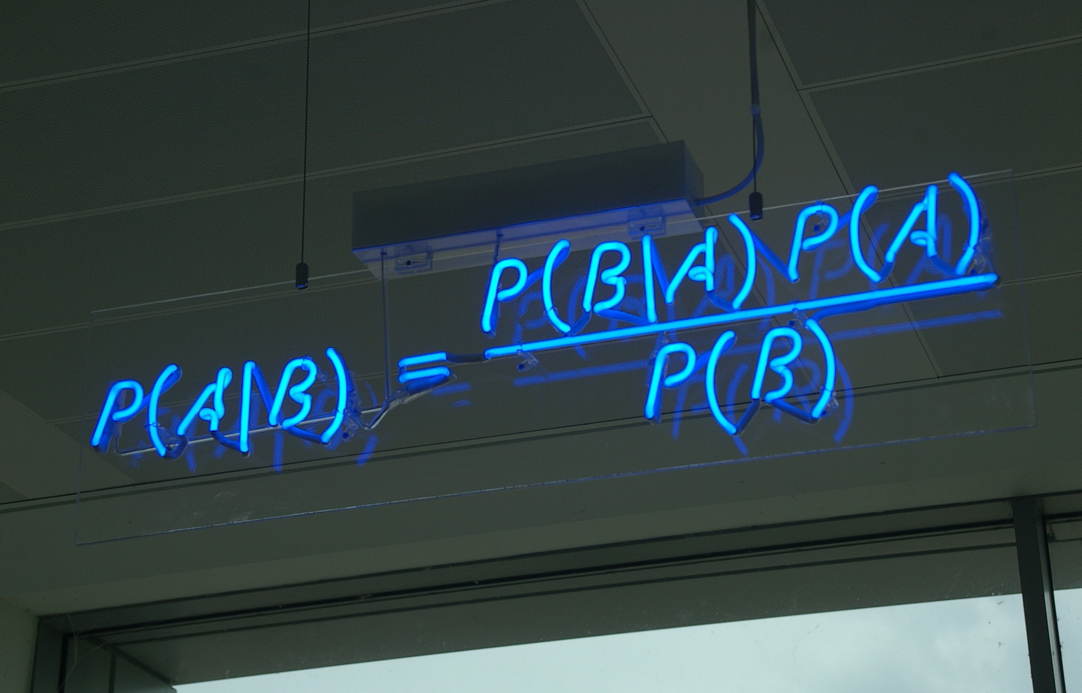
The posterior distribution is equal to the joint distribution divided by the marginal distribution of the evidence.
$$ \color{red}{P(\theta\ |\ \mathcal{D})} = \frac{\color{blue}{P(\mathcal{D}\ |\ \theta)\ P(\theta)}}{\color{green}{P(\mathcal{D})}} = \frac{\color{blue}{P(\mathcal{D}, \theta)}}{\color{green}{\int P(\mathcal{D}\ |\ \theta)\ P(\theta)\ d\theta}} $$For many useful models the marginal distribution of the evidence is hard or impossible to calculate analytically.
Modes of Bayesian Inference
- Conjugate models with closed-form posteriors
- Markov chain Monte Carlo algorithms
- Approximate Bayesian computation
- Distributional approximations
- Laplace approximations, INLA
- Variational inference
Markov Chain Monte Carlo Algorithms
- Construct a Markov chain whose stationary distribution is the posterior distribution
- Sample from the Markov chain for a long time
- Approximate posterior quantities using the empirical distribution of the samples
HTML(mcmc_video)
Beta-Binomial Model
We observe three successes in ten trials, and want to infer the true success probability.
x_beta_binomial = np.array([1, 1, 1, 0, 0, 0, 0, 0, 0, 0])
import pymc3 as pm

with pm.Model() as beta_binomial_model:
    p_beta_binomial = pm.Uniform('p', 0., 1.)
Applied interval-transform to p and added transformed p_interval_ to model.
with beta_binomial_model:
    x_obs = pm.Bernoulli('y', p_beta_binomial,
                         observed=x_beta_binomial)
fig

with beta_binomial_model:
    beta_binomial_trace_ = pm.sample(BETA_BINOMIAL_SAMPLES, random_seed=SEED)

beta_binomial_trace = beta_binomial_trace_[BETA_BINOMIAL_BURN::BETA_BINOMIAL_THIN]
Assigned NUTS to p_interval_
 [-------100%-------] 50000 of 50000 in 13.1 sec. | SPS: 3829.8 | ETA: 0.0
fig

Pros
- Asymptotically unbiased: converges to the true posterior afer many samples
- Model-agnostic algorithms
- Well-studied for more than 60 years
Cons
- Can take a long time to converge
- Can be difficult to assess convergence
- Difficult to scale
Variational Inference
- Choose a class of approximating distributions
- Find the best approximation to the true posterior
Variational inference minimizes the Kullback-Leibler divergence
$$\mathbb{KL}(\color{purple}{q(\theta)} \parallel \color{red}{p(\theta\ |\ \mathcal{D})}) = \mathbb{E}_q\left(\log\left(\frac{\color{purple}{q(\theta)}}{\color{red}{p(\theta\ |\ \mathcal{D})}}\right)\right)$$from approximate distributons, but we can't calculate the true posterior distribution.
Minimizing the Kullback-Leibler divergence
$$ \mathbb{KL}(\color{purple}{q(\theta)} \parallel \color{red}{p(\theta\ |\ \mathcal{D})}) = -(\underbrace{\mathbb{E}_q(\log \color{blue}{p(\mathcal{D}, \theta))} - \mathbb{E}_q(\color{purple}{\log q(\theta)})}_{\color{orange}{\textrm{ELBO}}}) + \log \color{green}{p(\mathcal{D})} $$is equivalent to maximizing the Evidence Lower BOund (ELBO), which only requires calculating the joint distribution.
Variational Inference Example
fig

Approximate the true distribution using a diagonal covariance Gaussian from the class
$$\mathcal{Q} = \left\{\left.N\left(\begin{pmatrix} \mu_x \\ \mu_y \end{pmatrix}, \begin{pmatrix} \sigma_x^2 & 0 \\ 0 & \sigma_y^2\end{pmatrix}\ \right|\ \mu_x, \mu_y \in \mathbb{R}^2, \sigma_x, \sigma_y > 0\right)\right\}$$fig

Pros
- A principled method to trade complexity for bias
- Optimization theory is applicable
- Assesment of convergence
- Scalability
Cons
- Biased estimate of the true posterior
- Better for prediction than interpretation
- Model-specific algorithms
Mean field variational inference
Assume the variational distribution factors independently as $q(\theta_1, \ldots, \theta_n) = q(\theta_1) \cdots q(\theta_n)$
The variational approximation can be found by coordinate ascent
$$ \begin{align*} q(\theta_i) & \propto \exp\left(\mathbb{E}_{q_{-i}}(\log(\mathcal{D}, \boldsymbol{\theta}))\right) \\ q_{-i}(\boldsymbol{\theta}) & = q(\theta_1) \cdots q(\theta_{i - 1})\ q(\theta_{i + 1}) \cdots q(\theta_n) \end{align*} $$Coordinate Ascent Cons
- Calculations are tedious, even when possible
- Convergence is slow when the number of parameters is large
Automating Variational Inference in Python
- Maximize ELBO using gradient ascent instead of coordinate ascent
- Tensor libraries calculate ELBO gradients automatically
Common themes
- Monte Carlo estimate of the ELBO gradient
- Minibatch estimates of the joint distribution
BBVI and ADVI arise from different ways of calculating the ELBO gradient

Beta-binomial model
import edward as ed
from edward.models import Bernoulli, Beta, Uniform

ed.set_seed(SEED)

# probability model
p = Uniform(a=0., b=1.)
x_edward_beta_binomial = Bernoulli(p=p)

data = {x_edward_beta_binomial: x_beta_binomial}
# variational approximation
q_p = Beta(a=tf_positive_variable(),
           b=tf_positive_variable())
q = {p: q_p}
%%time
beta_binomial_inference = ed.MFVI(q, data)
beta_binomial_inference.run(n_iter=10000, n_print=None)
CPU times: user 5.83 s, sys: 880 ms, total: 6.71 s
Wall time: 4.63 s
fig

from edward.models import PyMC3Model

# probability model
x_beta_binomial_obs = shared(np.zeros(1))

with pm.Model() as beta_binomial_model_untransformed:
    p = pm.Uniform('p', 0., 1., transform=None)
    x_beta_binomial_ = pm.Bernoulli('x', p, observed=x_beta_binomial_obs)

pymc3_data = {x_beta_binomial_obs: x_beta_binomial}
pymc3_beta_binomial_model = PyMC3Model(beta_binomial_model_untransformed)
%%time
# variational distribution
pymc3_q_p = Beta(a=tf_positive_variable(),
                 b=tf_positive_variable())
pymc3_q = {'p': pymc3_q_p}

pymc3_beta_binomial_inference = ed.MFVI(pymc3_q, pymc3_data,
                                        pymc3_beta_binomial_model)
pymc3_beta_binomial_inference.run(n_iter=30000, n_print=None)
CPU times: user 29.3 s, sys: 5.54 s, total: 34.8 s
Wall time: 22.4 s
fig

Edward-supported modeling "languages"
Direction density calculations
|
Congressional Ideal Points
vote_df.head()
| party | 0 | 1 | 2 | 3 | 4 | 5 | 6 | 7 | 8 | 9 | 10 | 11 | 12 | 13 | 14 | 15 | |
|---|---|---|---|---|---|---|---|---|---|---|---|---|---|---|---|---|---|
| rep | |||||||||||||||||
| 0 | 0 | 0 | 1 | 0 | 1 | 1 | 1 | 0 | 0 | 0 | 1 | NaN | 1 | 1 | 1 | 0 | 1 |
| 1 | 0 | 0 | 1 | 0 | 1 | 1 | 1 | 0 | 0 | 0 | 0 | 0 | 1 | 1 | 1 | 0 | NaN |
| 2 | 1 | NaN | 1 | 1 | NaN | 1 | 1 | 0 | 0 | 0 | 0 | 1 | 0 | 1 | 1 | 0 | 0 |
| 3 | 1 | 0 | 1 | 1 | 0 | NaN | 1 | 0 | 0 | 0 | 0 | 1 | 0 | 1 | 0 | 0 | 1 |
| 4 | 1 | 1 | 1 | 1 | 0 | 1 | 1 | 0 | 0 | 0 | 0 | 1 | NaN | 1 | 1 | 1 | 1 |
grid.fig

Idea:
- Representatives ($\color{blue}{\alpha_i}$) and bills ($\color{green}{\beta_j}$) each have an ideal point on a spectrum of conservativity
- If a representative's and bill's ideal points are the same, the representative has a 50% chance of voting for the bill
- Bills also have an ability to discriminate ($\color{red}{\gamma_j}$) between conservative and liberal representatives
- Some bills have broad bipartisan support, while some provoke votes along party lines
Representative ideal points
$$ \begin{align*} \color{blue}{\alpha_1}, \ldots, \color{blue}{\alpha_N} & \sim N(0, 1) \end{align*} $$def normal_log_prior(value, loc=0., scale=1.):
return tf.reduce_sum(normal.log_pdf(value, loc, scale))
Bill ideal points and discriminative abilities
$$ \begin{align*} \mu_{\beta} & \sim N(0, 1) \\ \sigma_{\beta} & \sim U(0, 1) \\ \color{green}{\beta_1}, \ldots, \color{green}{\beta_K} & \sim N(\mu_{\beta}, \sigma_{\beta}^2) \end{align*} $$$$ \begin{align*} \mu_{\gamma} & \sim N(0, 1) \\ \sigma_{\gamma} & \sim U(0, 1) \\ \color{red}{\gamma_1}, \ldots, \color{red}{\gamma_K} & \sim N(\mu_{\gamma}, \sigma_{\gamma}^2) \end{align*} $$
def hierarchical_log_prior(value, mu, sigma):
    log_hyperprior = normal_log_prior(mu) + uniform.log_pdf(sigma, 0., 1.)

    return log_hyperprior + normal_log_prior(value, loc=mu, scale=sigma)
Observation model
$$ \begin{align*} \mathbb{P}(\textrm{Representative }i \textrm{ votes for bill }j\ |\ \color{blue}{\alpha_i}, \color{green}{\beta_j}, \color{red}{\gamma_j}) & = \frac{1}{1 + \exp(-\color{red}{\gamma_j} \left(\color{blue}{\alpha_i} - \color{green}{\beta_j}\right))} \end{align*} $$def log_like(vote, rep, bill, alpha, beta, gamma):
# alpha, beta, and gamma have one entry for representative/bill,
# index them to have one entry per representative/bill combination
alpha_long = long_from_indices(alpha, rep)
beta_long = long_from_indices(beta, bill)
gamma_long = long_from_indices(gamma, bill)
p = tf.sigmoid(gamma_long * (alpha_long - beta_long))
return tf.reduce_sum(bernoulli.logpmf(vote, p))
Edward model
class IdealPoint:
    def log_prob(self, xs, zs):
        """
        xs is a dictionary of observed data
        zs is a dictionary of parameters

        Calculates the model's log joint distribution
        """
        # parameters
        alpha, beta, gamma = zs['alpha'], zs['beta'], zs['gamma']
        mu_beta, mu_gamma = zs['mu_beta'], zs['mu_gamma']
        sigma_beta, sigma_gamma = zs['sigma_beta'], zs['sigma_gamma']

        # observed data
        vote, bill, rep = xs['vote'], xs['bill'], xs['rep']

        # log joint distribution
        log_prior_ = log_prior(alpha,
                               beta, mu_beta, sigma_beta,
                               gamma, mu_gamma, sigma_gamma)
        log_like_ = log_like(vote, rep, bill,
                             alpha, beta, gamma)

        return log_prior_ + log_like_

ideal_point_model = IdealPoint()
BBVI inference
# variational distribution
q_alpha = tf_normal((n_reps,))

q_mu_beta = tf_normal()
q_sigma_beta = tf_uniform()
q_beta = tf_normal((N_BILLS,))

q_mu_gamma = tf_normal()
q_sigma_gamma = tf_uniform()
q_gamma = tf_normal((N_BILLS,))

q = {
    'alpha': q_alpha,
    'beta': q_beta, 'mu_beta': q_mu_beta, 'sigma_beta': q_sigma_beta,
    'gamma': q_gamma, 'mu_gamma': q_mu_gamma, 'sigma_gamma': q_sigma_gamma,
}
%%time
inference = ed.MFVI(q, ideal_point_data, ideal_point_model)
inference.run(n_iter=20000, n_print=None)
CPU times: user 1min 33s, sys: 30.2 s, total: 2min 4s
Wall time: 52.8 s
fig

Fun project: Recreate the Martin-Quinn dynamic ideal point model for ideology of U.S. Supreme Court justices with Edward

Variational Inference with PyMC3
Automatic Differentiation Variational Inference (ADVI)
- Only applicable to differentiable probability models
- Transform constrained parameters to be unconstrained
- Approximate the posterior for unconstrained parameters with mean field Gaussian
Beta-binomial model
Transformed distributions
fig

%%time
with beta_binomial_model:
    advi_fit = pm.advi(n=20000, random_seed=SEED)
Iteration 0 [0%]: ELBO = -10.91
Iteration 2000 [10%]: Average ELBO = -7.76
Iteration 4000 [20%]: Average ELBO = -7.37
Iteration 6000 [30%]: Average ELBO = -7.24
Iteration 8000 [40%]: Average ELBO = -7.22
Iteration 10000 [50%]: Average ELBO = -7.17
Iteration 12000 [60%]: Average ELBO = -7.15
Iteration 14000 [70%]: Average ELBO = -7.19
Iteration 16000 [80%]: Average ELBO = -7.18
Iteration 18000 [90%]: Average ELBO = -7.19
Finished [100%]: Average ELBO = -7.2
CPU times: user 3.12 s, sys: 0 ns, total: 3.12 s
Wall time: 3.1 s
ADVI approxiation to transformed posterior
fig

ADVI approximation to posterior
fig

Dependent Density Regression
fig

Idea: A mixture of linear models, where the unknown number of mixture weights depend on $x$
fig

Mixture weights
The model has infinitely many mixture components, we truncate to $K$
$$ \begin{align*} \alpha_1, \ldots, \alpha_K & \sim N(0, 1) \\ \beta_1, \ldots, \beta_K & \sim N(0, 1) \\ \boldsymbol{\pi} \ |\ \boldsymbol{\alpha}, \boldsymbol{\beta}, x & \sim \textrm{Logit-Stick-Breaking}(\boldsymbol{\alpha} + \boldsymbol{\beta} x) \\ \end{align*} $$K = 20
x_lidar = shared(std_range, broadcastable=(False, True))
with pm.Model() as lidar_model:
alpha = pm.Normal('alpha', 0., 1., shape=K)
beta = pm.Normal('beta', 0., 1., shape=K)
v = tt.nnet.sigmoid(alpha + beta * x_lidar)
pi = pm.Deterministic('pi', stick_breaking(v))
Component linear models
$$ \begin{align*} \gamma_1, \ldots, \gamma_K & \sim N(0, 100) \\ \delta_1, \ldots, \delta_K & \sim N(0, 100) \\ \tau_1, \ldots, \tau_K & \sim \textrm{Gamma}(1, 1) \\ Y_i\ |\ \gamma_i, \delta_i, \tau_i, x & \sim N(\gamma_i + \delta_i x, \tau_i^{-1}) \end{align*} $$with lidar_model:
gamma = pm.Normal('gamma', 0., 100., shape=K)
delta = pm.Normal('delta', 0., 100., shape=K)
tau = pm.Gamma('tau', 1., 1., shape=K)
ys = pm.Deterministic('ys', gamma + delta * x_lidar)
Applied log-transform to tau and added transformed tau_log_ to model.
Observation model
$$ \begin{align*} Y\ |\ \boldsymbol{\alpha}, \boldsymbol{\beta}, \boldsymbol{\gamma}, \boldsymbol{\delta}, \boldsymbol{\tau}, x & = \sum_{i = 1}^K \pi_i Y_i \\ \end{align*} $$with lidar_model:
lidar_obs = NormalMixture('lidar_obs', pi, ys, tau,
observed=std_logratio)
ADVI inference
%%time
N_ADVI_ITER = 50000

with lidar_model:
    advi_fit = pm.advi(n=N_ADVI_ITER, random_seed=SEED)
Iteration 0 [0%]: ELBO = -1173858.35
Iteration 5000 [10%]: Average ELBO = -1472209.86
Iteration 10000 [20%]: Average ELBO = -893902.97
Iteration 15000 [30%]: Average ELBO = -665586.63
Iteration 20000 [40%]: Average ELBO = -369517.75
Iteration 25000 [50%]: Average ELBO = 12058.54
Iteration 30000 [60%]: Average ELBO = 130100.63
Iteration 35000 [70%]: Average ELBO = 186668.28
Iteration 40000 [80%]: Average ELBO = 222983.67
Iteration 45000 [90%]: Average ELBO = 253507.05
Finished [100%]: Average ELBO = 266985.1
CPU times: user 43.7 s, sys: 0 ns, total: 43.7 s
Wall time: 43.7 s
fig

Posterior predictions
PPC_SAMPLES = 5000

lidar_ppc_x = np.linspace(std_range.min() - 0.05,
                          std_range.max() + 0.05,
                          100)

with lidar_model:
    # sample from the variational posterior distribution
    advi_trace = pm.sample_vp(advi_fit, PPC_SAMPLES, random_seed=SEED)

    # sample from the posterior predictive distribution
    x_lidar.set_value(lidar_ppc_x[:, np.newaxis])
    advi_ppc_trace = pm.sample_ppc(advi_trace, PPC_SAMPLES, random_seed=SEED)
Impact of truncation
fig

fig

References
Edward
PyMC3
http://pymc-devs.github.io/pymc3/
PyMC3 port of Probabilistic Programming and Bayesian Methods for Hackers
Variational Inference
Angelino, Elaine, Matthew James Johnson, and Ryan P. Adams. "Patterns of Scalable Bayesian Inference." arXiv preprint arXiv:1602.05221 (2016).
Blei, David M., Alp Kucukelbir, and Jon D. McAuliffe. "Variational inference: A review for statisticians." arXiv preprint arXiv:1601.00670 (2016).
Kucukelbir, Alp, et al. "Automatic Differentiation Variational Inference." arXiv preprint arXiv:1603.00788 (2016).
Ranganath, Rajesh, Sean Gerrish, and David M. Blei. "[Black Box Variational Inference]((http://www.cs.columbia.edu/~blei/papers/RanganathGerrishBlei2014.pdf)." AISTATS. 2014.
Models
Bafumi, Joseph, et al. "Practical issues in implementing and understanding Bayesian ideal point estimation." Political Analysis 13.2 (2005): 171-187.
Fox, Jean-Paul. Bayesian item response modeling: Theory and applications. Springer Science & Business Media, 2010.
Gelman, Andrew, et al. Bayesian data analysis. Vol. 2. Boca Raton, FL, USA: Chapman & Hall/CRC, 2014.
Gelman, Andrew, and Jennifer Hill. Data analysis using regression and multilevel/hierarchical models. Cambridge University Press, 2006.
Ren, Lu, et al. "Logistic stick-breaking process." Journal of Machine Learning Research 12.Jan (2011): 203-239.
Thank You!
@AustinRochford — Monetate Labs
arochford@monetate.com

The Jupyter notebook these slides were generated from is available here