![]()
Python Machine Learning Quick Tour¶
這份快速導覽主要介紹:
- 機器學習有哪些任務?
- 使用那些適當的 Python 工具完成任務?
順利執行這個筆記本的必要的套件如下:
| 工具函式庫套件 | 網址 |
|---|---|
numpy |
numpy.org |
scipy |
scipy.org |
matplotlib |
matplotlib.org |
seaborn |
seaborn.pydata.org |
pandas |
pandas.pydata.org |
scikit-learn |
scikit-learn.org |
"""
如果你已經裝好必要的Python套件環境的話,這份notebook可以在自己的電腦上執行。不然,可以使用Google的Colab。

若在Colab上開啟,請執行以下步驟:
1. 按右上角的【連線】,啟動雲端的Linux虛擬機器環境。
2. 執行這一格的程式碼,以安裝必要的套件。
"""
# 目前所有必要的套件在Colab上都有,這一格可以不用執行
!python --version
!pip list

# 日後若發現缺了某個套件,可以用 !pip install <套件名稱> 安裝
二元分類 - Binary Classification¶
§ Breast Cancer Wisconsin 資料集¶
資料來源是公開的乳癌資料集 UCI ML Breast Cancer Wisconsin (Diagnostic) dataset,檔案是逗號分隔欄位值的格式(Comma-Separated Values, CSV),一般文字編輯器或 Excel 都可以開啟,在 Python 的程式裡可以使用 pandas 套件來操作。
# 載入 pandas 套件
import pandas as pd

# 載入 WDBC (Wisconsin Diagnostic Breast Cancer) 資料集,傳回 pandas.DataFrame 類別的物件
dfWDBC = pd.read_csv('https://archive.ics.uci.edu/ml/machine-learning-databases/breast-cancer-wisconsin/wdbc.data', header=None)
# 資料欄位基本檢視
dfWDBC.info()
<class 'pandas.core.frame.DataFrame'>
RangeIndex: 569 entries, 0 to 568
Data columns (total 32 columns):
 #   Column  Non-Null Count  Dtype
---  ------  --------------  -----
 0   0       569 non-null    int64
 1   1       569 non-null    object
 2   2       569 non-null    float64
 3   3       569 non-null    float64
 4   4       569 non-null    float64
 5   5       569 non-null    float64
 6   6       569 non-null    float64
 7   7       569 non-null    float64
 8   8       569 non-null    float64
 9   9       569 non-null    float64
 10  10      569 non-null    float64
 11  11      569 non-null    float64
 12  12      569 non-null    float64
 13  13      569 non-null    float64
 14  14      569 non-null    float64
 15  15      569 non-null    float64
 16  16      569 non-null    float64
 17  17      569 non-null    float64
 18  18      569 non-null    float64
 19  19      569 non-null    float64
 20  20      569 non-null    float64
 21  21      569 non-null    float64
 22  22      569 non-null    float64
 23  23      569 non-null    float64
 24  24      569 non-null    float64
 25  25      569 non-null    float64
 26  26      569 non-null    float64
 27  27      569 non-null    float64
 28  28      569 non-null    float64
 29  29      569 non-null    float64
 30  30      569 non-null    float64
 31  31      569 non-null    float64
dtypes: float64(30), int64(1), object(1)
memory usage: 142.4+ KB
§ WDBC 資料集欄位說明¶
原始數據沒有包含欄位名稱,說明在另外一個檔案 "wdbc.names" 中。
- 欄位1: 樣本 ID
- 欄位2: 診斷結果,"M" = malignant 惡性,"B" = benign 良性
十個實數值的細胞核特徵由細針抽吸(fine needle aspiration cytology)的細胞病理影像樣本計算而來:
- 半徑 radius (mean of distances from center to points on the perimeter)
- 紋理 texture (standard deviation of gray-scale values)
- 周長 perimeter
- 面積 area
- 形狀平滑度 smoothness (local variation in radius lengths)
- 緊密度 compactness (perimeter^2 / area - 1.0)
- 輪廓凹陷度 concavity (severity of concave portions of the contour)
- 輪廓凹陷點 concave points (number of concave portions of the contour)
- 對稱性 symmetry
- 碎形維度 fractal dimension ("coastline approximation" - 1)
每個影像的這十個特徵都分別計算 mean,standard error,以及 worst(三個最大值的平均),共 30 個特徵欄位。

★ 觀念 ★¶
當然可以使用 Excel 來手動為原始數據檔案加上欄位名稱,或是訓練預測模型之前的前處理,但是所有的操作必須遵循以下原則:
- 保留原始檔案,修改的內容另存新檔。
- 記錄所有修改步驟及歷程,說明的內容要可以從原始檔案重現修改的結果。
要符合這樣的原則,使用 Python 程式進行處理還是首選。
# 說明中描述的欄位名稱
column_mean = [
    "radius_mean", "texture_mean", "perimeter_mean", "area_mean", "smoothness_mean",
    "compactness_mean", "concavity_mean", "concave points_mean", "symmetry_mean", "fractal_dimension_mean"
]
column_se = [
    "radius_se", "texture_se", "perimeter_se", "area_se", "smoothness_se",
    "compactness_se", "concavity_se", "concave points_se", "symmetry_se", "fractal_dimension_se"
]
column_worst = [
    "radius_worst", "texture_worst", "perimeter_worst", "area_worst", "smoothness_worst",
    "compactness_worst", "concavity_worst", "concave points_worst", "symmetry_worst", "fractal_dimension_worst"
]

column_names = ["id", "diagnosis"] + column_mean + column_se + column_worst

# 指定欄位名稱
dfWDBC.columns = column_names

# 再一次資料欄位基本檢視
dfWDBC.info()
<class 'pandas.core.frame.DataFrame'>
RangeIndex: 569 entries, 0 to 568
Data columns (total 32 columns):
 #   Column                   Non-Null Count  Dtype
---  ------                   --------------  -----
 0   id                       569 non-null    int64
 1   diagnosis                569 non-null    object
 2   radius_mean              569 non-null    float64
 3   texture_mean             569 non-null    float64
 4   perimeter_mean           569 non-null    float64
 5   area_mean                569 non-null    float64
 6   smoothness_mean          569 non-null    float64
 7   compactness_mean         569 non-null    float64
 8   concavity_mean           569 non-null    float64
 9   concave points_mean      569 non-null    float64
 10  symmetry_mean            569 non-null    float64
 11  fractal_dimension_mean   569 non-null    float64
 12  radius_se                569 non-null    float64
 13  texture_se               569 non-null    float64
 14  perimeter_se             569 non-null    float64
 15  area_se                  569 non-null    float64
 16  smoothness_se            569 non-null    float64
 17  compactness_se           569 non-null    float64
 18  concavity_se             569 non-null    float64
 19  concave points_se        569 non-null    float64
 20  symmetry_se              569 non-null    float64
 21  fractal_dimension_se     569 non-null    float64
 22  radius_worst             569 non-null    float64
 23  texture_worst            569 non-null    float64
 24  perimeter_worst          569 non-null    float64
 25  area_worst               569 non-null    float64
 26  smoothness_worst         569 non-null    float64
 27  compactness_worst        569 non-null    float64
 28  concavity_worst          569 non-null    float64
 29  concave points_worst     569 non-null    float64
 30  symmetry_worst           569 non-null    float64
 31  fractal_dimension_worst  569 non-null    float64
dtypes: float64(30), int64(1), object(1)
memory usage: 142.4+ KB
§ 觀察數據內容¶
一般而言,機器學習關心的是要如何從已知的資料中,建構一個可以用來預測未知資料特性的模型。 執行學習的任務使用電腦系統的演算法來*自動發現數據的規律性*,稱為模式識別(Pattern Recognition)。 所以機器學習演算法的設計,所關心的是如何識別資料中隱含的模式來作推論,而不是明確指示推論的邏輯。
然而,目前機器學習的技術還沒發展到可以完全自動的程度,開始訓練模型之前還有很多的前處理工作需要人的介入,不同的模型可能需要不同的數據前處理,所以首先要先觀察手上的資料,並盡可能了解每個欄位的意義以及跟預測目標的關聯,決定要做什麼必要的前處理:
- 哪些是特徵欄位 X? 哪些是目標欄位 Y? 有沒有多餘的不要進入模型訓練的欄位?
- 都是連續數值欄位嗎? 有沒有類別欄位?
- 有沒有漏失數據? 有沒有空值要填補或插補?
- 數值欄位的數值分布狀況? 要怎麼正規化?
- 目標類別分布狀況如何? 數量是否平均?
- 特徵與目標之間是否有線性或其他形式的相關?
- 各特徵之間是否有線性或其他形式的相關?
# 看一下前面幾筆,檢視資料內容
dfWDBC.head(5)
| id | diagnosis | radius_mean | texture_mean | perimeter_mean | area_mean | smoothness_mean | compactness_mean | concavity_mean | concave points_mean | ... | radius_worst | texture_worst | perimeter_worst | area_worst | smoothness_worst | compactness_worst | concavity_worst | concave points_worst | symmetry_worst | fractal_dimension_worst | |
|---|---|---|---|---|---|---|---|---|---|---|---|---|---|---|---|---|---|---|---|---|---|
| 0 | 842302 | M | 17.99 | 10.38 | 122.80 | 1001.0 | 0.11840 | 0.27760 | 0.3001 | 0.14710 | ... | 25.38 | 17.33 | 184.60 | 2019.0 | 0.1622 | 0.6656 | 0.7119 | 0.2654 | 0.4601 | 0.11890 |
| 1 | 842517 | M | 20.57 | 17.77 | 132.90 | 1326.0 | 0.08474 | 0.07864 | 0.0869 | 0.07017 | ... | 24.99 | 23.41 | 158.80 | 1956.0 | 0.1238 | 0.1866 | 0.2416 | 0.1860 | 0.2750 | 0.08902 |
| 2 | 84300903 | M | 19.69 | 21.25 | 130.00 | 1203.0 | 0.10960 | 0.15990 | 0.1974 | 0.12790 | ... | 23.57 | 25.53 | 152.50 | 1709.0 | 0.1444 | 0.4245 | 0.4504 | 0.2430 | 0.3613 | 0.08758 |
| 3 | 84348301 | M | 11.42 | 20.38 | 77.58 | 386.1 | 0.14250 | 0.28390 | 0.2414 | 0.10520 | ... | 14.91 | 26.50 | 98.87 | 567.7 | 0.2098 | 0.8663 | 0.6869 | 0.2575 | 0.6638 | 0.17300 |
| 4 | 84358402 | M | 20.29 | 14.34 | 135.10 | 1297.0 | 0.10030 | 0.13280 | 0.1980 | 0.10430 | ... | 22.54 | 16.67 | 152.20 | 1575.0 | 0.1374 | 0.2050 | 0.4000 | 0.1625 | 0.2364 | 0.07678 |
5 rows × 32 columns
# 丟掉不需要的 "id" 欄位
dfWDBC.drop(columns=['id'], inplace=True)
# 觀察目標類別數量分布狀況
print('\n-- 不同樣本值的出現次數:\n', dfWDBC.loc[:, ['diagnosis']].value_counts())
print('\n-- 所有不是N/A的樣本數:\n', dfWDBC.loc[:, ['diagnosis']].count())

# 也可以用序號存取 diagnosis 欄位
# 注意: id 欄位刪除後, diagnosis 變成第一個欄位
print('\n-- 不同樣本值的出現次數:\n', dfWDBC.iloc[:, 0].value_counts())
print('\n-- 所有不是N/A的樣本數:\n', dfWDBC.iloc[:, 0].count())

# 觀察: 惡性的類別比較少
print('\n-- 良性與惡性的樣本數比例:\n', dfWDBC.loc[:,'diagnosis'].value_counts() / dfWDBC.loc[:,'diagnosis'].count())
-- 不同樣本值的出現次數:
 diagnosis
B            357
M            212
dtype: int64

-- 所有不是N/A的樣本數:
 diagnosis    569
dtype: int64

-- 不同樣本值的出現次數:
 B    357
M    212
Name: diagnosis, dtype: int64

-- 所有不是N/A的樣本數:
 569

-- 良性與惡性的樣本數比例:
 B    0.627417
M    0.372583
Name: diagnosis, dtype: float64
★ 觀念 ★¶
資料集中時常會包含類別數據(Categorical Data),如 WDBC 資料集中"diagnosis"欄位值是"B"或"M"的字元,機器學習的演算法處理的都是數值,需要將類別數據轉成數值型態。
# 將 diagnosis 欄位良性與惡性的類別轉為 0 與 1
dfWDBC.loc[:,'diagnosis'] = dfWDBC.loc[:,'diagnosis'].map({'B':0, 'M':1})

# 檢視幾筆確認轉換結果沒問題
dfWDBC.iloc[-5:, :8]
| diagnosis | radius_mean | texture_mean | perimeter_mean | area_mean | smoothness_mean | compactness_mean | concavity_mean | |
|---|---|---|---|---|---|---|---|---|
| 564 | 1 | 21.56 | 22.39 | 142.00 | 1479.0 | 0.11100 | 0.11590 | 0.24390 |
| 565 | 1 | 20.13 | 28.25 | 131.20 | 1261.0 | 0.09780 | 0.10340 | 0.14400 |
| 566 | 1 | 16.60 | 28.08 | 108.30 | 858.1 | 0.08455 | 0.10230 | 0.09251 |
| 567 | 1 | 20.60 | 29.33 | 140.10 | 1265.0 | 0.11780 | 0.27700 | 0.35140 |
| 568 | 0 | 7.76 | 24.54 | 47.92 | 181.0 | 0.05263 | 0.04362 | 0.00000 |
# 各數值欄位的基本統計分布狀況
display(dfWDBC.loc[:,column_mean].describe())
display(dfWDBC.loc[:,column_se].describe())
display(dfWDBC.loc[:,column_worst].describe())

# 觀察: 數據 scale 差異大
| radius_mean | texture_mean | perimeter_mean | area_mean | smoothness_mean | compactness_mean | concavity_mean | concave points_mean | symmetry_mean | fractal_dimension_mean | |
|---|---|---|---|---|---|---|---|---|---|---|
| count | 569.000000 | 569.000000 | 569.000000 | 569.000000 | 569.000000 | 569.000000 | 569.000000 | 569.000000 | 569.000000 | 569.000000 |
| mean | 14.127292 | 19.289649 | 91.969033 | 654.889104 | 0.096360 | 0.104341 | 0.088799 | 0.048919 | 0.181162 | 0.062798 |
| std | 3.524049 | 4.301036 | 24.298981 | 351.914129 | 0.014064 | 0.052813 | 0.079720 | 0.038803 | 0.027414 | 0.007060 |
| min | 6.981000 | 9.710000 | 43.790000 | 143.500000 | 0.052630 | 0.019380 | 0.000000 | 0.000000 | 0.106000 | 0.049960 |
| 25% | 11.700000 | 16.170000 | 75.170000 | 420.300000 | 0.086370 | 0.064920 | 0.029560 | 0.020310 | 0.161900 | 0.057700 |
| 50% | 13.370000 | 18.840000 | 86.240000 | 551.100000 | 0.095870 | 0.092630 | 0.061540 | 0.033500 | 0.179200 | 0.061540 |
| 75% | 15.780000 | 21.800000 | 104.100000 | 782.700000 | 0.105300 | 0.130400 | 0.130700 | 0.074000 | 0.195700 | 0.066120 |
| max | 28.110000 | 39.280000 | 188.500000 | 2501.000000 | 0.163400 | 0.345400 | 0.426800 | 0.201200 | 0.304000 | 0.097440 |
| radius_se | texture_se | perimeter_se | area_se | smoothness_se | compactness_se | concavity_se | concave points_se | symmetry_se | fractal_dimension_se | |
|---|---|---|---|---|---|---|---|---|---|---|
| count | 569.000000 | 569.000000 | 569.000000 | 569.000000 | 569.000000 | 569.000000 | 569.000000 | 569.000000 | 569.000000 | 569.000000 |
| mean | 0.405172 | 1.216853 | 2.866059 | 40.337079 | 0.007041 | 0.025478 | 0.031894 | 0.011796 | 0.020542 | 0.003795 |
| std | 0.277313 | 0.551648 | 2.021855 | 45.491006 | 0.003003 | 0.017908 | 0.030186 | 0.006170 | 0.008266 | 0.002646 |
| min | 0.111500 | 0.360200 | 0.757000 | 6.802000 | 0.001713 | 0.002252 | 0.000000 | 0.000000 | 0.007882 | 0.000895 |
| 25% | 0.232400 | 0.833900 | 1.606000 | 17.850000 | 0.005169 | 0.013080 | 0.015090 | 0.007638 | 0.015160 | 0.002248 |
| 50% | 0.324200 | 1.108000 | 2.287000 | 24.530000 | 0.006380 | 0.020450 | 0.025890 | 0.010930 | 0.018730 | 0.003187 |
| 75% | 0.478900 | 1.474000 | 3.357000 | 45.190000 | 0.008146 | 0.032450 | 0.042050 | 0.014710 | 0.023480 | 0.004558 |
| max | 2.873000 | 4.885000 | 21.980000 | 542.200000 | 0.031130 | 0.135400 | 0.396000 | 0.052790 | 0.078950 | 0.029840 |
| radius_worst | texture_worst | perimeter_worst | area_worst | smoothness_worst | compactness_worst | concavity_worst | concave points_worst | symmetry_worst | fractal_dimension_worst | |
|---|---|---|---|---|---|---|---|---|---|---|
| count | 569.000000 | 569.000000 | 569.000000 | 569.000000 | 569.000000 | 569.000000 | 569.000000 | 569.000000 | 569.000000 | 569.000000 |
| mean | 16.269190 | 25.677223 | 107.261213 | 880.583128 | 0.132369 | 0.254265 | 0.272188 | 0.114606 | 0.290076 | 0.083946 |
| std | 4.833242 | 6.146258 | 33.602542 | 569.356993 | 0.022832 | 0.157336 | 0.208624 | 0.065732 | 0.061867 | 0.018061 |
| min | 7.930000 | 12.020000 | 50.410000 | 185.200000 | 0.071170 | 0.027290 | 0.000000 | 0.000000 | 0.156500 | 0.055040 |
| 25% | 13.010000 | 21.080000 | 84.110000 | 515.300000 | 0.116600 | 0.147200 | 0.114500 | 0.064930 | 0.250400 | 0.071460 |
| 50% | 14.970000 | 25.410000 | 97.660000 | 686.500000 | 0.131300 | 0.211900 | 0.226700 | 0.099930 | 0.282200 | 0.080040 |
| 75% | 18.790000 | 29.720000 | 125.400000 | 1084.000000 | 0.146000 | 0.339100 | 0.382900 | 0.161400 | 0.317900 | 0.092080 |
| max | 36.040000 | 49.540000 | 251.200000 | 4254.000000 | 0.222600 | 1.058000 | 1.252000 | 0.291000 | 0.663800 | 0.207500 |
★ 觀念 ★¶
數據的尺度差異大,直覺是尺度大的數字變化比較大,對決策的判斷會影響比較大,而實際上有很多機器學習的模型真的會受尺度大小的影響。 大多數的資料集都有尺度差異的現象,所以開始訓練預測模型之前,時常會先對數據進行正規化(Normalization),指的就是將數據調整到相同的尺度。
§ Logistic Regression¶
Logistic Regression 是線性的分類模型(不是回歸),預測結果的可能性是擬合 logistic (sigmoid) 函數的模型。
logistic(x)=11+e−x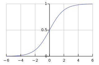
★ 觀念 ★¶
機器學習的手法是使用資料集 X 來調整匹配模型的參數,在監督式學習裡,每筆 X 資料都有已知的對應類別 Y,所執行的學習演算法可以表示為 ˆY=f(X),最後的 f(X) 函數模型是透過 訓練(training) 的過程來決定,也稱為 學習(learning)。
# 準備好 X 與 Y
Y = dfWDBC.loc[:,'diagnosis']
X = dfWDBC.drop(columns=['diagnosis'])

print('X shape = {}, Y shape = {}\n'.format(X.shape, Y.shape))
X shape = (569, 30), Y shape = (569,)
至此,只有丟掉不需要的欄位,把預測目標Y的類別轉為數值,X還沒做正規化或其他前處理。 不過有些機器學習的模型不受資料尺度差異的影響,直接先訓練看看來當作後續處理方法的評估基準,這也是常見的手法。 我們利用*Scikit-Learn*提供的工具來訓練 Logistic Regression 的模型。
from sklearn.linear_model import LogisticRegression

# 使用預設參數建構 LogisticRegression 模型物件
lrmodel = LogisticRegression()

# 用物件的 fit() 方法來訓練模型
lrmodel.fit(X, Y)
C:\RnD\miniconda3\lib\site-packages\sklearn\linear_model\_logistic.py:763: ConvergenceWarning: lbfgs failed to converge (status=1):
STOP: TOTAL NO. of ITERATIONS REACHED LIMIT.

Increase the number of iterations (max_iter) or scale the data as shown in:
    https://scikit-learn.org/stable/modules/preprocessing.html
Please also refer to the documentation for alternative solver options:
    https://scikit-learn.org/stable/modules/linear_model.html#logistic-regression
  n_iter_i = _check_optimize_result(
LogisticRegression()
有些機器學習的模型不受資料尺度差異的影響,看來 Logistic Regression 不是這樣的模型,最好還是先做一下正規化。
§ 正規化 Normalization¶
常用正規化類別如下:
sklearn.preprocessing.MinMaxScaler: 一般通用型正規化,尺度調整至 [0, 1] 區間。sklearn.preprocessing.StandardScaler: 又稱標準化(z-score),尺度調整至 mean 為 0 的單位標準差區間範圍。
對應的正規化函式如下:
from sklearn.preprocessing import scale

# 重新建構新的模型物件,用正規化過的 X 再訓練一次
lrmodel = LogisticRegression().fit(scale(X), Y)

# 看看訓練的如何
print('Accuracy = {:.2f}'.format(lrmodel.score(scale(X), Y)))
Accuracy = 0.99
模型確效 Model Validation¶
模型訓練後,要有方法來度量模型的預測品質。 在上一個範例的二元分類裡,模型訓練後輸出了一個分類正確率(Accuracy)的指標,但是計算分數的輸入是原始的訓練集X,所以只能用來表示模型可以被訓練起來。 機器學習希望建立的是能夠預測真實世界資料(real-world data)的模型,因此訓練資料越多越好,但最終我們還是只能從有限的取樣資料中來擬合真實世界的模型,而實際進行預測的資料不會跟用來訓練的資料一模一樣,因此模型準確度的評估應該使用另外一個(不是用來訓練模型的)資料集。
機器學習裡通常的做法是把資料分成兩份,一份訓練集(training set),另外一份完全不參與模型訓練的測試集(test set),最後模型的準確度只使用測試集來評估。 實際在訓練過程中,我們仍然希望所有的訓練集都可以用來訓練,同時也能有效地評估訓練過程參數的改變所影響的模型的效力,因此常用的折衷方式是把訓練集拆成 k 個小段(k-fold),每次都只保留其中某一段作驗證,其餘的作訓練,全部小段都同樣輪流作一次,然後把 k 次的結果作平均。 這樣就所有的資料都有訓練過也驗證過,這種交叉驗證的手法我們稱為 k-Fold Cross-Validation。

上圖中將訓練集切割為五段,每一段包含所有訓練集的其中 20%,這樣我們稱為 5-fold。 因為沒有浪費任何資料,這樣的交叉驗證方式可以更精準的評估學習模型的效能。 缺點是 k 次的交叉驗證要花比較久的時間運算,所以如果是如百萬筆等級的大型資料集,隨機抽樣 1% 都還有個一萬筆,這樣就可以不需要 k-fold。 至於要選擇幾個 k 的 fold 則沒有一定的準則,通常還是觀察訓練集的大小來決定,若是非常小的訓練集甚至可以採取 leave-one-out(共 n 筆作 n-fold)的特殊作法。
Scikit-learn 將交叉驗證的工具放在 model_selection 模組中,常用的如下:
from sklearn.model_selection import train_test_split

# 分割成訓練集和測試集
X_train, X_test, Y_train, Y_test = train_test_split(X, Y, test_size=0.2)
§ 數據洩漏¶
將資料集切割出訓練集和測試集以及進行k-fold交叉驗證時,必須注意避免數據洩漏(data leakage)的問題。
簡單地說,k-fold進行驗證的驗證集資料特徵,或是最後進行模型驗證的測試集資料特徵,都不能在訓練集訓練時被偷學到。 數據洩漏通常發生在資料的前處理過程,例如資料缺值的填補、或是數據的正規化等,套用這些處理時經常要先取得資料集的統計特徵(如平均值、標準差),像這樣的前處理不能在資料集分割前處理,否則結果會導致驗證時精準的假象,實際用來預測新資料時卻非常的不準。
Scikit-learn 提供一個 pipeline 的工具,可以用來簡化工作的流程:
- 先把個別處理步驟的方法分別定義好。
- 將負責處理每個步驟的物件,按照順序放進流程清單,學習模型物件放最後。
- 對資料集都套用指定的(前)處理,而且會避免數據洩漏的問題。
sklearn.pipeline.Pipeline(steps)- steps: 是工作流程的清單,照工作順序放 (name, transform) 的 tuple 的清單,最後一個一定要是 estimator。
from sklearn.pipeline import Pipeline
from sklearn.preprocessing import StandardScaler
# 使用已經內建交叉驗證的 Logistic Regression
from sklearn.linear_model import LogisticRegressionCV

lrcvmodel = Pipeline(
    steps=[
        ('zscaler', StandardScaler()),
        ('lrcv', LogisticRegressionCV(cv=10, max_iter=300, n_jobs=-1))
    ]
)

# 直接用 pipeline 來訓練,自動套用指定的正規化前處理
lrcvmodel.fit(X_train, Y_train)

# 測試模型的準確度
print('Accuracy = {:.2f}'.format(lrcvmodel.score(X_test, Y_test)))
Accuracy = 0.99
from sklearn.metrics import (
    accuracy_score,
    recall_score,
    roc_auc_score,
    confusion_matrix
)

Y_predict = lrcvmodel.predict(X_test)

# confusion matrix
TN, FP, FN, TP = confusion_matrix(Y_test, Y_predict).ravel()
print('\n[Confusion Matrix]:\n  | TP: {} | FP: {} |\n  | FN: {} | TN: {} |'.format(TP, FP, FN, TN))

# sensitivity & specificity
sensitivity = recall_score(Y_test, Y_predict, pos_label=1)
specificity = recall_score(Y_test, Y_predict, pos_label=0)
print('\n[Testing Scores]:\n  * Sensitivity: {:.3f}\n  * Specificity: {:.3f}'.format(sensitivity, specificity))
[Confusion Matrix]:
  | TP: 42 | FP: 0 |
  | FN: 1 | TN: 71 |

[Testing Scores]:
  * Sensitivity: 0.977
  * Specificity: 1.000
特徵選取¶
§ 相關係數¶
統計上有幾種常用的相關係數,一般提到相關係數指的都是 Pearson相關係數 r。
- Pearson相關係數度量兩個數列 x 和 y 之間的線性相關程度。
- 相關係數 r 的值介於 [-1, 1] 之間。
- r=1 表示完全線性匹配的正相關,y 在一條直線上隨著 x 增加而增加。
- r=0 表示x 和 y 之間沒有線性相關性。
- r=−1 表示完全線性匹配的負相關,y 在一條直線上隨著 x 增加而減少。
- r 值大小與關係強弱的對應解釋方式沒有標準,需考慮變數實際意義上的度量精度。
- 除了觀察 r 值大小,同時也應該要檢驗 "假設沒有關係" 的推論的 p-value 顯著性。
- 相關係數不受變數的尺度差異影響,正規化與否相關性不改變。
Pandas.DataFrame 有提供 corr() 的方法,預設就是 Pearson 相關係數,可以用來在 seaborn.heatmap上視覺化顯示。 若需要 p-value 的計算結果,可以使用 scypy.stats 模組的 pearsonr() 函數。
# 繪圖環境設定
%matplotlib inline
import matplotlib.pyplot as plt
plt.style.use('seaborn-darkgrid')
plt.rcParams['figure.figsize'] = (10.0, 8.0)

import seaborn as sns
# 各特徵值與診斷結果相關性(corr 預設是 Pearson 的相關係數)
plt.figure(figsize=(5, 10))
sns.heatmap(dfWDBC.corr().loc[:,['diagnosis']], annot=True, vmin=-1, vmax=1)
<AxesSubplot:>

# 各特徵值之間的相關性(corr 預設是 Pearson 的相關係數)
plt.figure(figsize=(16, 12))
sns.heatmap(dfWDBC.corr(), annot=True, square=True, vmin=-1, vmax=1)
<AxesSubplot:>

很多資料集的數據不是常態分佈,欄位之間也很難有線性關係。 在 WDBC 資料集中,我們很幸運地可以觀察到有些特徵值與診斷結果有線性相關,特徵與特徵兩兩之間也出現一些高度相關的。 根據相關係數觀察到的現象,可以用來篩選特徵(feature selection),以降低特徵的維度,有效的特徵篩選通常可以讓模型更容易訓練,泛化能力更好。
- 首先丟掉與目標欄位相關性非常低的特徵(如: −0.2≤r≤0.2),保留相關性高的特徵。
- 保留下來相關性高的特徵中,有出現兩兩高度相關的(如: r>0.9),很可能去掉其中一個對模型的預測能力影響不大。
§ 其他特徵處理¶
沒有一種指標適用所有的資料特性,有時需要嘗試不同的指標或選取方法才能找到適合資料特性的方法。 有些方法不是透過指標選取,而是將特徵轉換或映射到不同的維度空間。