§ 使用 numpy 套件¶
# 載入 numpy 的慣例方式
import numpy as np
# 部份範例會將資料視覺化,預先開啟 matplotlib 互動呈現
%matplotlib inline
import matplotlib.pyplot as plt
§ 取得說明¶
除了官方文件 (https://numpy.org/doc/stable/ ) 以外,互動式介面下也可以取得說明。
# 取得 np.array 的說明
np.array?
# 忘記函式的全名怎麼拼,可以打前幾個字,然後按 Tab 鍵。
np.con
11.1 建立向量、矩陣、與陣列¶
Numpy 的 ndarray 是可以存放同類型資料的多維度陣列,在大多數的應用中,陣列元素的資料類型通常是數值。ndarray 類型的物件可以透過 array()、zeros()、ones()、或 identity() 等函式建立。 描述 ndarray 的基本的屬性有:
ndarray.ndim- 維度ndarray.shape- Tuple 表示每個維度的大小,也可以指定新的 Tuple 值改變陣列的形狀,類似reshape()函式,差別是shape屬性是就地改變。ndarray.size- 元素總數量ndarray.dtype- 元素資料形態,數值通常使用 numpy 提供的np.float64、np.int32、np.int16、 ...等,可以只寫float、int使用系統預設的浮點數或整數型態。
# a one-dimension vector
v = np.array([0, 1, 2, 3])

print('v: ndim={}, shape={}, size={}, dtype={}'.format(v.ndim, v.shape, v.size, v.dtype))
v: ndim=1, shape=(4,), size=4, dtype=int32
# a 1 x 4 row vector/matrix,明確指定使用整數型態的資料
rowv = np.array([[0, 1, 2, 3]], dtype=int)

print('rowv: ndim={}, shape={}, size={}, dtype={}'.format(rowv.ndim, rowv.shape, rowv.size, rowv.dtype))
rowv: ndim=2, shape=(1, 4), size=4, dtype=int32
# a 4 x 1 column vector/matrix,明確指定使用浮點數型態的資料
colv = np.array([[0],
                 [1],
                 [2],
                 [3]], dtype=float)

print('colv: ndim={}, shape={}, size={}, dtype={}'.format(colv.ndim, colv.shape, colv.size, colv.dtype))
colv: ndim=2, shape=(4, 1), size=4, dtype=float64
# a 3 x 4 matrix,明確指定使用 np.float64 浮點數型態的資料
Amat = np.array([[0, 1,  2,  3],
                 [4, 5,  6,  7],
                 [8, 9, 10, 11]], dtype=np.float64)

print('Amat: ndim={}, shape={}, size={}, dtype={}'.format(Amat.ndim, Amat.shape, Amat.size, Amat.dtype))
Amat: ndim=2, shape=(3, 4), size=12, dtype=float64
# a 2 x 3 x 4 array
A3d = np.array([[[ 0,  1,  2,  3],
                 [ 4,  5,  6,  7],
                 [ 8,  9, 10, 11]],

                [[12, 13, 14, 15],
                 [16, 17, 18, 19],
                 [20, 21, 22, 23]]])

print('A3d: ndim={}, shape={}, size={}, dtype={}'.format(A3d.ndim, A3d.shape, A3d.size, A3d.dtype))
A3d: ndim=3, shape=(2, 3, 4), size=24, dtype=int32
# 元素都為 0 的 3 x 3 matrix
np.zeros((3, 3))
array([[0., 0., 0.],
       [0., 0., 0.],
       [0., 0., 0.]])
# 元素都為 1 的 4 x 4 matrix
np.ones((4, 4))
array([[1., 1., 1., 1.],
       [1., 1., 1., 1.],
       [1., 1., 1., 1.],
       [1., 1., 1., 1.]])
# 5 x 5 identity matrix
np.identity(5)
array([[1., 0., 0., 0., 0.],
       [0., 1., 0., 0., 0.],
       [0., 0., 1., 0., 0.],
       [0., 0., 0., 1., 0.],
       [0., 0., 0., 0., 1.]])
其他常用函式,可用來建立具備某種規律排列數列的 ndarray:
np.arange- 產生一維的固定間距的整數數列陣列。 類似 Python 內建函式range()的 numpy 陣列版。np.linspace- 在指定區間內產生線性(固定)間隔的指定數量的數列。np.logspace- 在指定區間內產生對數間隔的指定數量的數列。np.random.rand- 產生指定大小的均勻分佈隨機亂數。np.random.randn- 產生指定大小的高斯分佈隨機亂數。np.random.randint-
產生指定大小的隨機整數。
# [0, 10) 整數數列
np.arange(10)
array([0, 1, 2, 3, 4, 5, 6, 7, 8, 9])
# 指定範圍及間距,arange([start, ]stop, [step, ]),注意參數 [start, stop) 為半開放區間
np.arange(1, 10, 2)
array([1, 3, 5, 7, 9])
# 時常用來產生數列後就轉成需要的維度形狀
np.arange(1, 25).reshape((2, 3, 4))
array([[[ 1,  2,  3,  4],
        [ 5,  6,  7,  8],
        [ 9, 10, 11, 12]],

       [[13, 14, 15, 16],
        [17, 18, 19, 20],
        [21, 22, 23, 24]]])
# 指定範圍及點數,linspace(start, stop, num=50),注意參數 [start, stop] 為封閉區間
linda = np.linspace(1, 10, num=9)
print(linda)
[ 1. 2.125 3.25 4.375 5.5 6.625 7.75 8.875 10. ]
# 指定範圍及點數,logspace(start, stop, num=50),注意參數 [start, stop] 為封閉區間
logda = np.logspace(0, 1, num=9)
print(logda)
[ 1.          1.33352143  1.77827941  2.37137371  3.16227766  4.21696503
  5.62341325  7.49894209 10.        ]
# visualize
y = linda
fig, ax = plt.subplots()
ax.plot(linda, y, 'o-')
ax.plot(logda, y, '*--')
[<matplotlib.lines.Line2D at 0x2c408b91cc0>]

# linspace 適合用來生成數列代入函數求得一系列的函數值
from numpy import pi
x = np.linspace(0, 2*pi, 100)
y = np.sin(x)

fig, ax = plt.subplots()
ax.plot(x, y)
[<matplotlib.lines.Line2D at 0x2c408bf9a58>]

# Uniform 分佈的隨機亂數
image = np.random.rand(30, 30)

# 二維的陣列資料都可以當成影像顯示
plt.imshow(image)
plt.colorbar()
<matplotlib.colorbar.Colorbar at 0x2c408cc45c0>

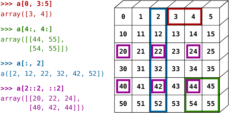
11.2 索引及片段 Indexing and Slicing¶
§ 基本索引與片段¶
ndarray 基本的索引和片段語法,與使用 Python 序列容器(如:List)的語法雷同,都是使用中括號內置索引序號或冒號間隔的片段範圍:
- 一維
vector[index],二維matrix[index1, index2],高維array[index1, index2, index3, ...]。 - 一維片段
vector[start:end:step],二維片段matrix[start:end:step, start:end:step],高維片段 array 類推。
片段的索引方式可以放在等號左邊,用來直接對原陣列的片段指派新的值。存取陣列的片段,返回的是原陣列裡的參考 view,不是複製一個新的陣列,如果明確需要另外複製一份相同內容的陣列,可以使用 copy 函式,np.copy() 或 ndarray.copy() 都可以用。
以下索引及片段示意圖來自 scipy-lectures.org
Amat = np.arange(12).reshape((3,4))
print('Amat =\n', Amat, '\n')
Amat =
 [[ 0  1  2  3]
 [ 4  5  6  7]
 [ 8  9 10 11]]
# 索引維度若小於實際維度時,返回的是子陣列的參考
Amat[0]
array([0, 1, 2, 3])
# 所以個別元素的存取,也可以使用另外一種效率較差的索引方式
print('Amat[0][2] = {},Amat[0, 2] = {},兩種索引方式存取同一個位置的元素,\n'
      '但 Amat[0][2] 效率較差,因為 Amat[0] 會先產生一個暫時的陣列物件才存取索引2元素。'
      .format(Amat[0][2], Amat[0, 2]))
Amat[0][2] = 2,Amat[0, 2] = 2,兩種索引方式存取同一個位置的元素,
但 Amat[0][2] 效率較差,因為 Amat[0] 會先產生一個暫時的陣列物件才存取索引2元素。
# 片段可以放在等號左邊,用來直接對原陣列的片段指派新的值
Amat[:, 1::2] = 7
Amat
array([[ 0,  7,  2,  7],
       [ 4,  7,  6,  7],
       [ 8,  7, 10,  7]])
# 明確複製新的物件
AsliceCopy = Amat[:, 1::2].copy()
# 更改元素值
AsliceCopy[:] = 9

# 不會更改到原陣列
print('Amat =\n', Amat, '\n')
print('AsliceCopy =\n', AsliceCopy)
Amat =
 [[ 0  7  2  7]
 [ 4  7  6  7]
 [ 8  7 10  7]]

AsliceCopy =
 [[9 9]
 [9 9]
 [9 9]]
§ 索引技巧 - 使用布林陣列¶
陣列索引的中括號裡可以使用另外一個相同形狀及大小的 boolean 陣列(元素都是 True 或 False 的 bool 型態陣列),這種用法的 boolean 陣列又稱為遮罩(mask),索引的結果,會返回“複製”索引結果的元素值的一維陣列。
如果遮罩陣列的維度比被索引的陣列還要少的時候,不足的維度視爲片段全選。 例如: 若 A 爲二維陣列,mask 是一維的遮罩,則 A[mask] 等同於 A[mask, :]。 若索引結果無法形成有效的陣列形狀,則視爲錯誤的陳述。
# 產生 [0, 255] 區間的亂數
I = np.random.randint(0, 256, size=(16,16))

# 準備將二維矩陣顯示成影像
fig1, ax1 = plt.subplots()
# 顯示原本的亂數影像
ax1.imshow(I, cmap='gray')
ax1.set_title('Original Image')
Text(0.5, 1.0, 'Original Image')

# 取門檻值後作為遮罩,"<" 的比較運算下在一節中詳細介紹
mask = I < 128
# 顯示遮罩成影像
fig2, ax2 = plt.subplots()
ax2.imshow(mask, cmap='gray')
ax2.set_title('Mask image')
Text(0.5, 1.0, 'Mask image')

# 遮罩陣列當成索引陣列,將原陣列中符合門檻值條件的元素都設成 0
I[mask] = 0
# 顯示修改後的二維矩陣成影像
fig3, ax3 = plt.subplots()
ax3.imshow(I, cmap='gray')
ax3.set_title('I[mask] set to 0')
Text(0.5, 1.0, 'I[mask] set to 0')

# 遮罩索引的結果,會返回索引結果的元素值的一維陣列
I[I > 250]
array([252, 253, 254, 255, 251])
# 5 x 7 陣列
Amat = np.arange(35).reshape(5,7)
print(Amat)
[[ 0  1  2  3  4  5  6]
 [ 7  8  9 10 11 12 13]
 [14 15 16 17 18 19 20]
 [21 22 23 24 25 26 27]
 [28 29 30 31 32 33 34]]
# 遮罩陣列比被索引陣列的維度還要少時,不足的維度視爲片段全選
mask = np.array([False, True, False, False, True])
Amat[mask]
array([[ 7,  8,  9, 10, 11, 12, 13],
       [28, 29, 30, 31, 32, 33, 34]])
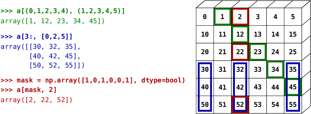
§ 索引技巧 - 使用整數索引陣列¶
整數索引陣列裡的整數就是索引的序號,正整數或負整數的規則與單一索引值相同。 在索引陣列中,相同的索引序號可以重複出現,其結果就是重複選取相同元素。
- 對一維的陣列而言,索引陣列會返回一個結果的陣列,其維度與索引陣列相同。
- 對高維的陣列而言,若索引陣列的維度比較少,不足的維度視爲片段全選。
- 片段、遮罩陣列、整數索引陣列可以同時穿插使用。
以下索引技巧及片段示意圖來自 scipy-lectures.org
v = np.arange(35)
print('v =', v)

# 一維索引陣列,注意索引陣列是 Python List
v[[7, 7, 21, 23, -7, -5]]
v = [ 0  1  2  3  4  5  6  7  8  9 10 11 12 13 14 15 16 17 18 19 20 21 22 23
 24 25 26 27 28 29 30 31 32 33 34]
array([ 7, 7, 21, 23, 28, 30])
# 返回索引結果與索引陣列維度及形狀相同
print(v[np.array([[7, 7], [21, 23], [-7, -5]])])
[[ 7  7]
 [21 23]
 [28 30]]
# 可以直接指派新值給這樣的索引位置
v[np.array([[7, 7], [21, 23], [-7, -5]])] = 99
print(v)
[ 0  1  2  3  4  5  6 99  8  9 10 11 12 13 14 15 16 17 18 19 20 99 22 99
 24 25 26 27 99 29 99 31 32 33 34]
# 索引陣列的維度比較少,不足的維度視爲片段全選
v.shape = (5, 7)
print(v)

v[np.array([1, 3, 4])]
[[ 0  1  2  3  4  5  6]
 [99  8  9 10 11 12 13]
 [14 15 16 17 18 19 20]
 [99 22 99 24 25 26 27]
 [99 29 99 31 32 33 34]]
array([[99,  8,  9, 10, 11, 12, 13],
       [99, 22, 99, 24, 25, 26, 27],
       [99, 29, 99, 31, 32, 33, 34]])
§ 一維平坦化 Flatten¶
Amat = np.array([[1, 2, 3], [4, 5, 6], [7, 8, 9]])
print('Amat =\n', Amat)

# 一維 row-major 平坦化,返回原陣列的 view(同物件參考)
print('Amat reshape =', Amat.reshape(-1))

# 一維 row-major 平坦化,返回原陣列的 copy
print('Amat flatten =', Amat.flatten())
Amat =
 [[1 2 3]
 [4 5 6]
 [7 8 9]]
Amat reshape = [1 2 3 4 5 6 7 8 9]
Amat flatten = [1 2 3 4 5 6 7 8 9]
§ 轉置 Transpose¶
# transpose
print('Amat.T =\n', Amat.T)
print('numpy.transpose(Amat) =\n', np.transpose(Amat))
Amat.T =
 [[1 4 7]
 [2 5 8]
 [3 6 9]]
numpy.transpose(Amat) =
 [[1 4 7]
 [2 5 8]
 [3 6 9]]
§ 增減維度¶
Aflat = Amat.reshape(-1)
print('Aflat shape{} = {}'.format(Aflat.shape, Aflat))
Aflat shape(9,) = [1 2 3 4 5 6 7 8 9]
# 擴增維度,以下操作與 Aflat[np.newaxis, :] 相同
#Aexp0 = np.expand_dims(Aflat, axis=0)
Aexp0 = Aflat[np.newaxis, :]
print('Aexp0 shape{} = {}'.format(Aexp0.shape, Aexp0))
Aexp0 shape(1, 9) = [[1 2 3 4 5 6 7 8 9]]
# 擴增維度,以下操作與 Aflat[:, np.newaxis] 相同
Aexp1 = np.expand_dims(Aflat, axis=1)
print('Aexp1 shape{} = {}'.format(Aexp1.shape, Aexp1))
Aexp1 shape(9, 1) = [[1]
 [2]
 [3]
 [4]
 [5]
 [6]
 [7]
 [8]
 [9]]
# 移除陣列的單一維度
Asqueeze = np.squeeze(Aexp0)
print('Aexp0 squeeze to {} = {}'.format(Asqueeze.shape, Asqueeze))
Aexp0 squeeze to (9,) = [1 2 3 4 5 6 7 8 9]
§ 堆疊、串接、重組¶
許多 numpy 操作或運算陣列的方法都有一個 axis 參數,例如以下範例中示範的 concatenate。 這個 axis 參數通常是用來指定該方法要套用的方向:
- 第一個維度(
axis=0)是列(row)方向或稱垂直(vertical)方向 - 第二個維度(
axis=1)的行(column)方向或稱水平(horizontal)方向 - 其他更高維度的方向(axis = 2, 3, 4, ...)
有的方法還可以使用 axis=None 的設定,這個無軸向的操作則視不同方法有不同的意義。
| row0 | col1 | col2 | col3 | col4 | ... | colN |
|---|---|---|---|---|---|---|
| row1 | ||||||
| row2 | ||||||
| row3 | ||||||
| row4 | ||||||
| ... | ||||||
| rowN |
# 建立一黑一白的 3 x 3 陣列
B, W = np.zeros((3,3)), np.ones((3,3))
print(B, '\n'); print(W, '\n')

# 沿水平方向串接
BnW = np.concatenate((B, W), axis=1)
print(BnW)
[[0. 0. 0.]
 [0. 0. 0.]
 [0. 0. 0.]]

[[1. 1. 1.]
 [1. 1. 1.]
 [1. 1. 1.]]

[[0. 0. 0. 1. 1. 1.]
 [0. 0. 0. 1. 1. 1.]
 [0. 0. 0. 1. 1. 1.]]
# 翻轉,用 axis 參數指定翻轉方向
WnB = np.flip(BnW, axis=1)
print(WnB, '\n')
[[1. 1. 1. 0. 0. 0.]
 [1. 1. 1. 0. 0. 0.]
 [1. 1. 1. 0. 0. 0.]]
# 沿垂直方向串接
BnW_WnB = np.concatenate((BnW, WnB), axis=0)
print(BnW_WnB)
[[0. 0. 0. 1. 1. 1.]
 [0. 0. 0. 1. 1. 1.]
 [0. 0. 0. 1. 1. 1.]
 [1. 1. 1. 0. 0. 0.]
 [1. 1. 1. 0. 0. 0.]
 [1. 1. 1. 0. 0. 0.]]
# 重複區塊如貼瓷磚
ChessBoard = np.tile(BnW_WnB, (2,2))
fig, ax = plt.subplots()
ax.imshow(ChessBoard, cmap='gray')
<matplotlib.image.AxesImage at 0x2c408ead048>

11.4 數值陣列運算¶
§ Element-wise 算數及比較運算¶
ndarray 常用的算數及比較運算操作是定義為對每個元素的逐項(element-wise)操作,然後返回運算結果的 ndarray 物件。
- 比較運算子 - 運算結果返回
bool陣列。
| 比較運算操作 | 說明 |
|---|---|
| X < Y | 小於 |
| X <= Y | 小於或等於 |
| X > Y | 大於 |
| X >= Y | 大於或等於 |
| X == Y | 等於 |
| X != Y | 不等於 |
| logical_and(X, Y) | 真值邏輯 AND |
| logical_or(X, Y) | 真值邏輯 OR |
| logical_xor(X, Y) | 真值邏輯 XOR |
| logical_not(X) | 真值邏輯 NOT |
Note: 要比較兩個陣列(array-wise)是否形狀大小及元素全部相同,可以使用 array_equal(X, Y) 函式。
- 算數運算子 - 運算結果返回數值陣列。
| 算數運算操作 | 說明 | in-place 操作 |
|---|---|---|
| X + Y, X - Y | 加法,減法 | +=, -= |
| **X * Y, X / Y** | 乘法,除法 | ***=, /=** |
| X // Y, X % Y | 取商,取餘數 | //=, %= |
| **X**Y** | 指數次方 | ****=** |
| X | Y, X & Y | 位元 OR,AND | |=, &= |
| X << Y, X >> Y | 位元左位移,右位移 | <<=, >>= |
| X ^ Y | 位元 XOR | ^= |
- 一元算數運算子 - 運算結果返回數值陣列。
| 算數運算操作 | 說明 |
|---|---|
| -X | 取負數 |
| ~X | 位元反相 |
# 元素逐項(element-wise)比較
a = np.array([1, 2, 3, 4])
b = np.array([4, 2, 2, 4])
print('a == b =>', a == b)
print('a > b =>', a > b)
a == b => [False  True False  True]
a > b => [False False  True False]
# 陣列整體(array-wise)比較
a = np.array([1, 2, 3, 4])
b = np.array([4, 2, 2, 4])
c = np.array([1, 2, 3, 4])
print('a, b 陣列是否完全相等:', np.array_equal(a, b))
print('a, c 陣列是否完全相等:', np.array_equal(a, c))
a, b 陣列是否完全相等: False
a, c 陣列是否完全相等: True
# 陣列真值邏輯比較
a = np.array([1, 1, 0, 0], dtype=bool)
b = np.array([1, 0, 1, 0], dtype=bool)
print('真值邏輯比較 a OR b:', np.logical_or(a, b))
print('真值邏輯比較 a AND b:', np.logical_and(a, b))
真值邏輯比較 a OR b: [ True  True  True False]
真值邏輯比較 a AND b: [ True False False False]
# 陣列元素逐項(element-wise)運算
a = np.array([1, 2, 3, 4])
b = np.array([4, 2, 2, 4])
c = np.array([1, 2, 3, 4])
print('a + b =', a + b)
print('b * c =', b * c)
print('a + b * c =', a + b * c)
print('(a + b) / c =', (a + b) / c)
a + b = [5 4 5 8]
b * c = [ 4  4  6 16]
a + b * c = [ 5  6  9 20]
(a + b) / c = [5.         2.         1.66666667 2.        ]
§ 散播 Broadcasting¶
上述二元運算的一般形式中,除了兩個陣列運算元(X, Y)的形狀大小都一致以外,numpy 也容許在符合散播(broadcasting)條件下運算元形狀大小不一樣。 基本的散播相容的規則是:
- 兩個陣列維度大小相等,或
- 其中有一個維度大小是 1。
以下散播機制的示意圖來自 scipy-lectures.org
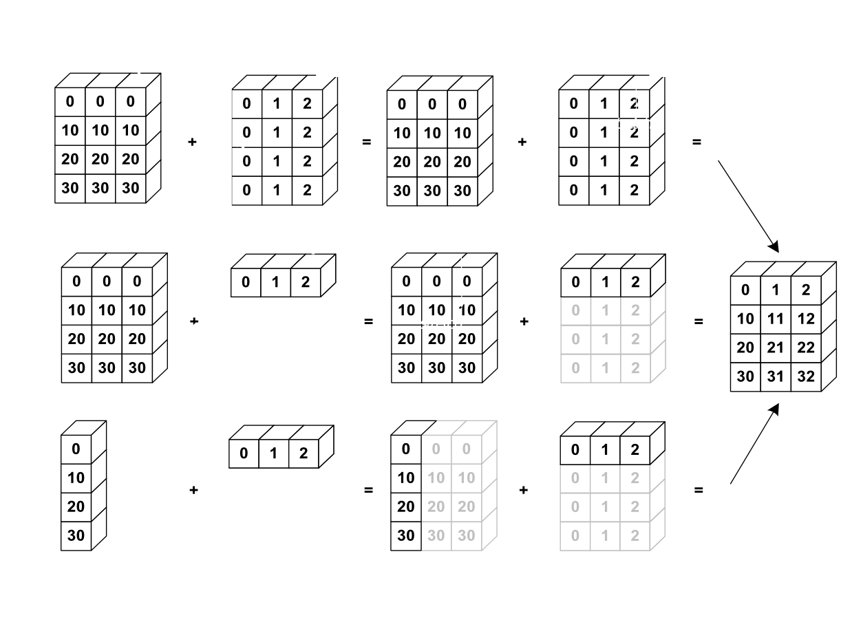
看似複雜的散播機制,其實都是為了簡化計算及程式碼的算式,讓程式碼更直覺、更自然、有更高的可讀性。以下範例及示意圖來自 numpy 官方手冊:
>>> a = array([1.0, 2.0, 3.0])
>>> b = 2.0
>>> a * b
array([ 2.,  4.,  6.])

Amat = np.arange(12).reshape(3, 4)
print(Amat)

# 之前看過的片段指派新值,其實暗中運用了 broadcasting
Amat[2] = 0
print(Amat)
[[ 0  1  2  3]
 [ 4  5  6  7]
 [ 8  9 10 11]]
[[0 1 2 3]
 [4 5 6 7]
 [0 0 0 0]]
# 計算距離
x, y = np.arange(6).reshape((6,1)), np.arange(6).reshape((1,6))
distance = np.sqrt(x ** 2 + y ** 2)
print(distance)
plt.pcolor(distance, cmap='jet')
plt.colorbar()
[[0.         1.         2.         3.         4.         5.        ]
 [1.         1.41421356 2.23606798 3.16227766 4.12310563 5.09901951]
 [2.         2.23606798 2.82842712 3.60555128 4.47213595 5.38516481]
 [3.         3.16227766 3.60555128 4.24264069 5.         5.83095189]
 [4.         4.12310563 4.47213595 5.         5.65685425 6.40312424]
 [5.         5.09901951 5.38516481 5.83095189 6.40312424 7.07106781]]
<matplotlib.colorbar.Colorbar at 0x2c408fdce10>

# 前一個計算距離的範例,使用 np.ogrid 可達到相同目的
x, y = np.ogrid[0:6, 0:6]
print(np.sqrt(x ** 2 + y ** 2))
x, y
[[0.         1.         2.         3.         4.         5.        ]
 [1.         1.41421356 2.23606798 3.16227766 4.12310563 5.09901951]
 [2.         2.23606798 2.82842712 3.60555128 4.47213595 5.38516481]
 [3.         3.16227766 3.60555128 4.24264069 5.         5.83095189]
 [4.         4.12310563 4.47213595 5.         5.65685425 6.40312424]
 [5.         5.09901951 5.38516481 5.83095189 6.40312424 7.07106781]]
(array([[0],
        [1],
        [2],
        [3],
        [4],
        [5]]), array([[0, 1, 2, 3, 4, 5]]))
# 不想要 broadcasting 的話,使用 np.mgrid 可達到相同目的
x, y = np.mgrid[0:6, 0:6]
print(np.sqrt(x ** 2 + y ** 2))
x, y
[[0.         1.         2.         3.         4.         5.        ]
 [1.         1.41421356 2.23606798 3.16227766 4.12310563 5.09901951]
 [2.         2.23606798 2.82842712 3.60555128 4.47213595 5.38516481]
 [3.         3.16227766 3.60555128 4.24264069 5.         5.83095189]
 [4.         4.12310563 4.47213595 5.         5.65685425 6.40312424]
 [5.         5.09901951 5.38516481 5.83095189 6.40312424 7.07106781]]
(array([[0, 0, 0, 0, 0, 0],
        [1, 1, 1, 1, 1, 1],
        [2, 2, 2, 2, 2, 2],
        [3, 3, 3, 3, 3, 3],
        [4, 4, 4, 4, 4, 4],
        [5, 5, 5, 5, 5, 5]]), array([[0, 1, 2, 3, 4, 5],
        [0, 1, 2, 3, 4, 5],
        [0, 1, 2, 3, 4, 5],
        [0, 1, 2, 3, 4, 5],
        [0, 1, 2, 3, 4, 5],
        [0, 1, 2, 3, 4, 5]]))
§ 有無向量運算優化的差異¶
對 list 裡的所有數值操作相同運算,免不了要使用迴圈。 使用 numpy.ndarray 運算,不僅程式碼的算式精簡、可讀性較高,還可以運用處理器的向量運算引擎,獲得更快的運算能力。
# 使用迴圈計算 10000 個整數加法
L = list(range(10000))
%timeit [x+1 for x in L]
509 µs ± 5.46 µs per loop (mean ± std. dev. of 7 runs, 1000 loops each)
# 使用 numpy 陣列的向量運算 10000 個整數加法
A = np.arange(10000, dtype=int)
%timeit A + 1
6.17 µs ± 125 ns per loop (mean ± std. dev. of 7 runs, 100000 loops each)
# 使用迴圈計算 10000 個浮點數指數運算
import random
L = [random.random() for x in range(10000)]
%timeit [x**2.0 for x in L]
1.46 ms ± 15.7 µs per loop (mean ± std. dev. of 7 runs, 1000 loops each)
# 使用 numpy 陣列的向量運算 10000 個浮點數指數運算
A = np.random.rand(10000)
%timeit A ** 2.0
4.58 µs ± 16.6 ns per loop (mean ± std. dev. of 7 runs, 100000 loops each)
# least-squares solution to a linear matrix equation
# 已知點座標 (x1,y1), (x2,y2), (x3,y3), (x4,y4), ...
x = np.array([0, 1, 2, 3])
y = np.array([-1, 0.2, 0.9, 2.1])
print('y =', y)

# 匹配直線方程式 y = mx + c (線性回歸)
# 將方程式重新改寫成陣列形式 y = Ap, where A = [x 1], p = [m c]'
A = np.vstack([x, np.ones(len(x))]).T
print('A =\n', A)

# 最小平方法解線性方程式最佳解
m, c = np.linalg.lstsq(A, y, rcond=None)[0]
print('\nsolution: m = {}, c = {}'.format(m, c))

fig, ax = plt.subplots()
ax.plot(x, y, 'o', label='Original data', markersize=10)
ax.plot(x, m*x + c, 'r', label='Fitted line')
ax.legend()
y = [-1.   0.2  0.9  2.1]
A =
 [[0. 1.]
 [1. 1.]
 [2. 1.]
 [3. 1.]]

solution: m = 0.9999999999999997, c = -0.949999999999999
<matplotlib.legend.Legend at 0x2c40904fb38>

作業練習¶
改寫上面的最小平方法範例,使用 arange() + random 雜訊產生 x, y 的測試資料,再執行求解方程式看看。