Improved Graph Laplacian via Geometric Self-Consistency
The github notebook viewer fails to render some plots in this notebook correctly, please view it on jupyter nbviewer.
The Task
- Problem: Estimate the
radiusof heat kernel in manifold embedding - Formally: Optimize Laplacian w.r.t. parameters (e.g.
radius) - Previous work:
- asymptotic rates depending on the (unknown) manifold [4]
- Embedding dependent neighborhood reconstruction [6]
- Challenge: it’s an unsupervised problem! What “target” to choose?
The radius affects…
- Quality of manifold embedding via neighborhood selection
- Laplacian-based embedding and clustering via the kernel for computing similarities
- Estimation of other geometric quantities that depend on the Laplacian (e.g Riemannian metric) or not (e.g intrinsic dimension).
- Regression on manifolds via Gaussian Processes or Laplacian regularization.
All the reference is the same as the poster.
Radius Estimation on hourglass dataset
In this tutorial, we are going to estimate the radius of a noisy hourglass data. The method we used is based on our NIPS 2017 paper "Improved Graph Laplacian via Geometric Self-Consistency" (Perrault-Joncas et. al). Main idea is to find an estimated radius $\hat{r}_d$ given dimension $d$ that minimize the distorsion. The distorsion is evaluated by the riemannian metrics of local tangent space.
Below are some configurations that enables plotly to render Latex properly.
import plotly
plotly.offline.init_notebook_mode(connected=True)

from IPython.core.display import display, HTML
display(HTML(
    '<script>'
        'var waitForPlotly = setInterval( function() {'
            'if( typeof(window.Plotly) !== "undefined" ){'
                'MathJax.Hub.Config({ SVG: { font: "STIX-Web" }, displayAlign: "center" });'
                'MathJax.Hub.Queue(["setRenderer", MathJax.Hub, "SVG"]);'
                'clearInterval(waitForPlotly);'
            '}}, 250 );'
    '</script>'
))
Generate data
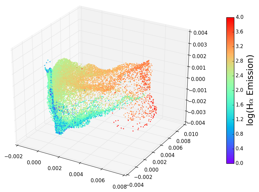
This dataset used in this tutorial has a shape of hourglass, with size = 10000 and dimension be 13. The first three dimensions of the data is generated by adding gaussian noises onto the noise-free hourglass data, with sigma_primary = 0.1, the variance of the noises added on hourglass data. We made addition_dims = 10, which is the addition noises dimension to make the whole dataset has dimension 13, with sigmal_additional = 0.1, which is the variance of additional dimension.
from plotly.offline import iplot
from megaman.datasets import generate_noisy_hourglass

data = generate_noisy_hourglass(size=10000, sigma_primary=0.1,
                                addition_dims=10, sigma_additional=0.1)
We can visualize dataset with the following plots:
from megaman.plotter.scatter_3d import scatter_plot3d_plotly
import plotly.graph_objs as go

t_data = scatter_plot3d_plotly(data,marker=dict(color='rgb(0, 102, 0)',opacity=0.5))
l_data = go.Layout(title='Noisy hourglass scatter plot for first 3 axis.')
f_data = go.Figure(data=t_data,layout=l_data)
iplot(f_data)
Radius estimation
To estimate the radius, we need to find the pairwise distance first.
To do so, we compute the adjacency matrix using the Geometry modules in megaman.
rmax=5
rmin=0.1

from megaman.geometry import Geometry

geom = Geometry(adjacency_method='brute',adjacency_kwds=dict(radius=rmax))
geom.set_data_matrix(data)
dist = geom.compute_adjacency_matrix()
For each data points, the distortion will be estimated. If the size $N$ used in estimating the distortion is large, it will be computationally expensive. We want to choose a sample with size $N'$ such that the average distion is well estimated. In our cases, we choose $N'=1000$. The error will be around $\frac{1}{\sqrt{1000}} \approx 0.03$.
In this example, we searched radius from the minimum pairwise distance rmin to the maximum distance between points rmax. By doing so, the distance matrix will be dense. If the matrix is too large to fit in the memory, smaller maximum radius rmax can be chosen to make the distance matrix sparse.
Based on the discussion above, we run radius estimation with
- sample size=1000 (created by choosing one data point out of every 10 of the original data.)
- radius search from
rmin=0.1tormax=50, with 50 points in logspace. - dimension
d=1
Specify run_parallel=True for searching the radius in parallel.
from megaman.utils.estimate_radius import run_estimate_radius
import numpy as np

# subsample by 10.
sample = np.arange(0,data.shape[0],10)

distorion_vs_rad_dim1 = run_estimate_radius(
    data, dist, sample=sample, d=1, rmin=rmin, rmax=rmax,
    ntry=50, run_parallel=True, search_space='logspace')
Run radius estimation same configurations as above except
- dimension
d=2
distorion_vs_rad_dim2 = run_estimate_radius(
    data, dist, sample=sample, d=2, rmin=0.1, rmax=5,
    ntry=50, run_parallel=True, search_space='logspace')
Radius estimation result
The estimated radius is the minimizer of the distorsion, denoted as $\hat{r}_{d=1}$ and $\hat{r}_{d=2}$. (In the code, it's est_rad_dim1 and est_rad_dim2)
distorsion_dim1 = distorion_vs_rad_dim1[:,1].astype('float64')
distorsion_dim2 = distorion_vs_rad_dim2[:,1].astype('float64')
rad_search_space = distorion_vs_rad_dim1[:,0].astype('float64')

argmin_d1 = np.argmin(distorsion_dim1)
argmin_d2 = np.argmin(distorsion_dim2)
est_rad_dim1 = rad_search_space[argmin_d1]
est_rad_dim2 = rad_search_space[argmin_d2]

print ('Estimated radius with d=1 is: {:.4f}'.format(est_rad_dim1))
print ('Estimated radius with d=2 is: {:.4f}'.format(est_rad_dim2))
Estimated radius with d=1 is: 1.0969
Estimated radius with d=2 is: 1.0128
Plot distorsions with different radii
t_distorsion = [go.Scatter(x=rad_search_space, y=distorsion_dim1, name='Dimension = 1'),
                go.Scatter(x=rad_search_space, y=distorsion_dim2, name='Dimension = 2')]

l_distorsion = go.Layout(
    title='Distorsions versus radii',
    xaxis=dict(
        title='$\\text{Radius } r$',
        type='log',
        autorange=True
    ),
    yaxis=dict(
        title='Distorsion',
        type='log',
        autorange=True
    ),
    annotations=[
        dict(
            x=np.log10(est_rad_dim1),
            y=np.log10(distorsion_dim1[argmin_d1]),
            xref='x',
            yref='y',
            text='$\\hat{r}_{d=1}$',
            font = dict(size = 30),
            showarrow=True,
            arrowhead=7,
            ax=0,
            ay=-30
        ),
        dict(
            x=np.log10(est_rad_dim2),
            y=np.log10(distorsion_dim2[argmin_d2]),
            xref='x',
            yref='y',
            text='$\\hat{r}_{d=2}$',
            font = dict(size = 30),
            showarrow=True,
            arrowhead=7,
            ax=0,
            ay=-30
        )
    ]
)
f_distorsion = go.Figure(data=t_distorsion,layout=l_distorsion)
iplot(f_distorsion)
Application to dimension estimation
We followed the method proposed by [Chen et. al (2011)]((http://lcsl.mit.edu/papers/che_lit_mag_ros_2011.pdf) [5] to verify the estimated radius reflect the truth intrinsic dimension of the data. The basic idea is to find the largest gap of singular value of local PCA, which correspond to the dimension of the local structure.
We first plot the average singular values versus radii.
from rad_est_utils import find_argmax_dimension, estimate_dimension
# rad_est_utils.py is located in https://github.com/mmp2/megaman/tree/master/examples

rad_search_space, singular_values = estimate_dimension(data, dist)
The singular gap is the different between two singular values. Since the intrinsic dimension is 2, we are interested in the region where the largest singular gap is the second. The region is:
singular_gap = -1*np.diff(singular_values,axis=1)
second_gap_is_max_range = (np.argmax(singular_gap,axis=1) == 1).nonzero()[0]
start_idx, end_idx = second_gap_is_max_range[0], second_gap_is_max_range[-1]+1

print ('The index which maximize the second singular gap is: {}'.format(second_gap_is_max_range))
print ('The start and end index of largest continuous range is {} and {}, respectively'.format(start_idx, end_idx))
The index which maximize the second singular gap is: [20 21 22 23 24 25 26 27 28 29 30 31 32 33]
The start and end index of largest continuous range is 20 and 34, respectively
Averaged singular values with different radii
Plot the averaged singular values with different radii. The gray shaded area is the continous range in which the largest singular gap is the second, (local structure has dimension equals 2). And the purple shaded area denotes the second singular gap.
By hovering the line on this plot, you can see the value of the singular gap.
from rad_est_utils import plot_singular_values_versus_radius, generate_layouts

t_avg_singular = plot_singular_values_versus_radius(singular_values, rad_search_space, start_idx, end_idx)
l_avg_singular = generate_layouts(start_idx, end_idx, est_rad_dim1, est_rad_dim2, rad_search_space)
f_avg_singular = go.Figure(data=t_avg_singular,layout=l_avg_singular)
iplot(f_avg_singular)
Histogram of estimated dimensions with estimated radius.
We first find out the estimated dimensions of each points in the data using the estimated radius $\hat{r}_{d=1}$ and $\hat{r}_{d=2}$.
dimension_freq_d1 = find_argmax_dimension(data,dist, est_rad_dim1)
dimension_freq_d2 = find_argmax_dimension(data,dist, est_rad_dim2)
The histogram of estimated dimensions with different optimal radius is shown as below:
t_hist_dim = [go.Histogram(x=dimension_freq_d1,name='d=1'),
            go.Histogram(x=dimension_freq_d2,name='d=2')]

l_hist_dim = go.Layout(
    title='Dimension histogram',
    xaxis=dict(
        title='Estimated dimension'
    ),
    yaxis=dict(
        title='Counts'
    ),
    bargap=0.2,
    bargroupgap=0.1
)

f_hist_dim = go.Figure(data=t_hist_dim,layout=l_hist_dim)

iplot(f_hist_dim)
Conclusion
- Choosing the correct radius/bound/scale is important in any non-linear dimension reduction task
- The Geometry Consistency (GC) Algorithm required minimal knowledge: maximum radius, minimum radius, (optionally: dimension $d$ of the manifold.)
- The chosen radius can be used in
- any embedding algorithm
- semi-supervised learning with Laplacian Regularizer (see our NIPS 2017 paper)
- estimating dimension $d$ (as shown here)
- The megaman python package is scalable, and efficient

Reference
[1] R. R. Coifman, S. Lafon. Diffusion maps. Applied and Computational Harmonic Analysis, 2006.
[2] D. Perrault-Joncas, M. Meila, Metric learning and manifolds: Preserving the intrinsic geometry , arXiv1305.7255
[3] X. Zhou, M. Belkin. Semi-supervised learning by higher order regularization. AISTAT, 2011
[4] A. Singer. From graph to manifold laplacian: the convergence rate. Applied and Computational Harmonic Analysis, 2006.
[5] G. Chen, A. Little, M. Maggioni, L. Rosasco. Some recent advances in multiscale geometric analysis of point clouds. Wavelets and multiscale analysis. Springer, 2011.
[6] L. Chen, A. Buja. Local Multidimensional Scaling for nonlinear dimension reduction, graph drawing and proximity analysis, JASA,2009.