![]()
Prof. Dr. -Ing. Gerald Schuller
Jupyter Notebook: Renato Profeta
# For Google Colab Only
try:
    import google.colab
    !pip uninstall plotly -y
    !pip install plotly==3.10.0

except Exception as e:
    print("Not inside Google Colab: %s. Using standard configurations." % (e))
Not inside Google Colab: No module named 'google'. Using standard configurations.
# For Google Colab Only
inColab=False
try:
    import google.colab
    import plotly.io as pio
    pio.renderers.default = 'colab'
    def enable_plotly_in_cell():
        import IPython
        from plotly.offline import init_notebook_mode
        display(IPython.core.display.HTML('''<script src="/static/components/requirejs/require.js"></script>'''))
        init_notebook_mode(connected=False)
    inColab=True

except Exception as e:
    print("Not inside Google Colab: %s. Using standard configurations." % (e))
Not inside Google Colab: No module named 'google'. Using standard configurations.
Quantization
%%html
<iframe width="560" height="315" src="https://www.youtube.com/embed/gFCjY9tNg3s" frameborder="0" allow="accelerometer; encrypted-media; gyroscope; picture-in-picture" allowfullscreen></iframe>
Quantization is the process of mapping a continuous range of values into a finite range of discrete values.
%%html
<iframe width="560" height="315" src="https://www.youtube.com/embed/HsiRKPK1Cag" frameborder="0" allow="accelerometer; encrypted-media; gyroscope; picture-in-picture" allowfullscreen></iframe>
Python Example
Assume our A/D converter has an input range of -1V to 1V, 4 bit accuracy (meaning we have a total of $2^4$ codewords or indices), and the A/D converter has 0.2 V at its input.
# Stepsize
range_max=1   # Maximum input range
range_min=-1  # Minumum input range
N=4           # Number of bits

stepsize=(range_max-range_min)/(2**N)
stepsize
0.125
Next we get quantization index which is then encoded as a codeword:
input_voltage=0.2
index =  round(input_voltage/stepsize)
index
2
Observe: If the quantization stepsize is constant, independent of the signal, we call it a “uniform quantizer”.
The index then is coded using the 4 bits and sent to a decoder, for instance using the 4 bit binary codeword “0010”. The first bit usually is the sign bit. The decoder reconstructs the voltage by first decoding the codeword to an index, and for instance by multiplying the index with the stepsize:
reconstr=stepsize*index
reconstr
0.25
This is also called the (de-)quantized signal, and its difference to the original value or signal is called the quantization error. In our example the quantization error is Quantized Value – Original Value = 0.25V-0.2V=0.05 V
**Observe:** There is always a range of voltages which is mapped to the same codeword. We call this range $\Delta$, or **stepsize**. These steps represent the quantization in the A/D conversion process, and they lead to quantization errors.
The output after quantization is a linear **“Pulse Code Modulation” (PCM)** signal. It is linear in the sense that the code values are proportional to the input signal values.
Quantization Error
%%html
<iframe width="560" height="315" src="https://www.youtube.com/embed/qgFSD5fKPaE" frameborder="0" allow="accelerometer; encrypted-media; gyroscope; picture-in-picture" allowfullscreen></iframe>
Let's now call our quantization error “e”. Then the quantization error power is the expectation value of the squared quantization error e:
where $p(e)$ is the probability of error value e. Here we compute the power of each possible error value e by squaring it, and multiply it with its probability to obtain the average power.
This number will give us some impression of the signal quality after quantization, if we set it in relation to the signal energy. Then we get a Signal to Noise Ratio (SNR) for our quantizer and A/D converter.
Assume the quantization error e is uniformly distributed (all possible values of the quantization error e appear with equal probability), which is usually the case if the signal is much larger than the quantization step size $\Delta$ (large signal condition). Since the integral over the probabilities of all possible values of e must be 1, and the possible values of e are between $-\Delta /2$ and $\Delta /2$,
we have
$$ \large p(e)=1/\Delta$$which yields
$$ \large E(e^2)=\frac{1} {\Delta} \cdot \int_ {-\Delta/2} ^ {\Delta/2} e^2 de = \frac{1} {\Delta} \left(\frac{(\Delta/2)^3} {3} - \frac{(-\Delta/2)^3} {3} \right) = \frac{\Delta^2}{12}$$Hence the quantization error power for a uniform quantizer with stepsize $\Delta$ and with a large signal is:
$$ \large E(e^2)=\frac{\Delta^2}{12} $$Mid-Rise and Mid-Tread Quantization
%%html
<iframe width="560" height="315" src="https://www.youtube.com/embed/XagP9ixzRAg" frameborder="0" allow="accelerometer; encrypted-media; gyroscope; picture-in-picture" allowfullscreen></iframe>
Depending on if the quantizer has the input voltage 0 at the center of a quantization interval or on the boundary of that interval, we call the quantizer a mid-tread or a mid rise quantiser, as illustrated in the following picture:
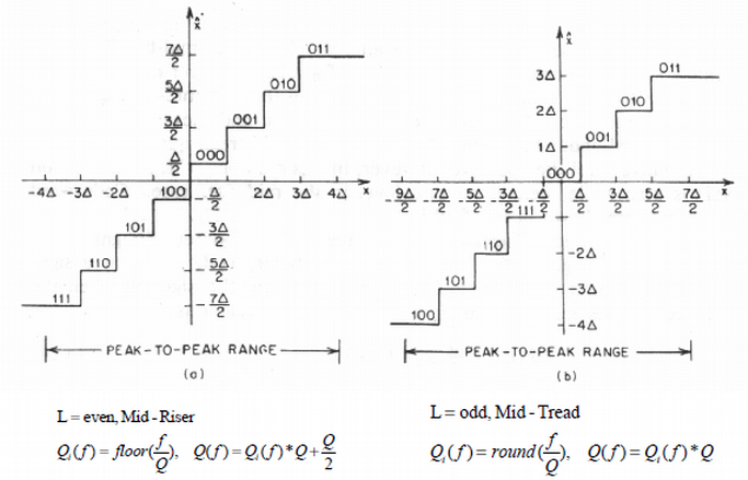
Here, $Q_i(f)$ is the index after quantization (which is then encoded and sent to the receiver), and Q(f) is the de-quantization, which produces the quantized reconstructed value at the receiver.
This makes mainly a difference at very small input values. For the mid-rise quantiser, very small values are always quantized to +/- half the quantization interval ($\pm \Delta/2$ ), whereas for the mid-tread quantizer, very small input values are always rounded to zero. You can also think about the mid-rise quantizer as not having a zero as a reconstruction value, but only very small positive and negative values.
So the mid-rise can be seen as more accurate, because it also reacts to very small input values, and the mid tread can be seen as saving bit-rate because it always quantizes very small values to zero.
Observe that the expectation of the quantization error power for large signals stays the same for both types.
Observe: the Mid-Tread quantizer “swallows” small signal levels, since they are all rounded to zero. The Mid-Rise quantizer still captures small levels, but distorted.
Python Example
%%html
<iframe width="560" height="315" src="https://www.youtube.com/embed/tnKeSKOmEz4" frameborder="0" allow="accelerometer; encrypted-media; gyroscope; picture-in-picture" allowfullscreen></iframe>
# Imports
import numpy as np
import matplotlib.pyplot as plt
import plotly.offline
import plotly.tools as tls
import plotly.plotly as py

# Configurations
plotly.offline.init_notebook_mode(connected=True)
import warnings; warnings.simplefilter('ignore')
# Signal Processing Parameters
Fs = 32000   # Sampling frequency
T=1/Fs       # Sampling Time
# Input Signal
A=1
freq=500
n_period=1
period=np.round((1/freq)*n_period*Fs).astype(int)
t = np.arange(Fs+1)*T # Time vector
sinewave = A*np.sin(2*np.pi*freq*t)
# Quantization and De-quantization
N=4
stepsize=(1.0-(-1.0))/(2**N)
#Encode
sinewave_quant_rise_ind=np.floor(sinewave/stepsize)
sinewave_quant_tread_ind=np.round(sinewave/stepsize)
#Decode
sinewave_quant_rise_rec=sinewave_quant_rise_ind*stepsize+stepsize/2
sinewave_quant_tread_rec=sinewave_quant_tread_ind*stepsize
# Shape for plotting
t_quant=np.delete(np.repeat(t[:period+1],2),-1)
sinewave_quant_rise_rec_plot=np.delete(np.repeat(sinewave_quant_rise_rec[:period+1],2),0)
sinewave_quant_tread_rec_plot=np.delete(np.repeat(sinewave_quant_tread_rec[:period+1],2),0)
# Quantization Error
quant_error_tread=sinewave_quant_tread_rec-sinewave
quant_error_rise=sinewave_quant_rise_rec-sinewave
#plot
if inColab:
    enable_plotly_in_cell()

fig = plt.figure(figsize=(12,8))
plt.subplot(2,1,1)
plt.plot(t[:period+1],sinewave[:period+1], label='Original Signal')
plt.plot(t_quant,sinewave_quant_rise_rec_plot, label='Quantized Signal (Mid-Rise)')
plt.plot(t_quant,sinewave_quant_tread_rec_plot, label='Quantized Signal (Mid-Tread)')
plt.title('Orignal and Quantized Signals', fontsize=18)
plt.xlabel('Time [s]')
plt.ylabel('Amplitude')
plt.yticks(np.arange(-1-stepsize, 1+stepsize, stepsize))
#plt.legend()
plt.grid()
#plt.tight_layout()
plt.subplot(2,1,2)
plt.plot(t[:period+1],quant_error_tread[:period+1], label='Quantization Error')
plt.grid()
plt.title('Quantization Error (Mid-Tread)', fontsize=18)
plt.xlabel('Time [s]')
plt.ylabel('Amplitude')
#plt.tight_layout()
plt.subplots_adjust(hspace=0.5)

plotly_fig = tls.mpl_to_plotly(fig)
plotly_fig.layout.update(showlegend=True)
plotly.offline.iplot(plotly_fig)
# Listen to Audio
import IPython.display as ipd
print('Orignal Signal')
ipd.display(ipd.Audio(sinewave, rate=Fs))
print('Quantized Signal (Mid-Tread)')
ipd.display(ipd.Audio(sinewave_quant_tread_rec, rate=Fs))
print('Quantized Signal (Mid-Rise)')
ipd.display(ipd.Audio(sinewave_quant_rise_rec, rate=Fs))
print('Quantization Error (Mid-Tread)')
ipd.display(ipd.Audio(quant_error_tread, rate=Fs))
print('Quantization Error (Mid-Rise)')
ipd.display(ipd.Audio(quant_error_rise, rate=Fs))
Orignal Signal
Quantized Signal (Mid-Tread)
Quantized Signal (Mid-Rise)
Quantization Error (Mid-Tread)
Quantization Error (Mid-Rise)
# Imports
from scipy.fftpack import fft
import plotly.offline
import plotly.tools as tls
import plotly.plotly as py

# Configurations
if inColab==False:
    plotly.offline.init_notebook_mode(connected=True)
else:
    enable_plotly_in_cell()

import warnings; warnings.simplefilter('ignore')

# Signal Processing Parameters
NFFT=2**10
#Frequency Analysis
freqs = np.fft.fftfreq(NFFT, d=T) # Frequency bins
original_fft=fft(sinewave, n=NFFT)
original_fft/=np.abs(original_fft).max()
quantized_tread_fft=fft(sinewave_quant_tread_rec, n=NFFT)
quantized_tread_fft/=np.abs(quantized_tread_fft).max()
quantized_rise_fft=fft(sinewave_quant_rise_rec, n=NFFT)
quantized_rise_fft/=np.abs(quantized_rise_fft).max()

# Plot
fig=plt.figure(figsize=(12,8))
plt.plot(freqs[0:NFFT//2],20*np.log10(np.abs(quantized_rise_fft[0:NFFT//2]).clip(min=1e-5)), label='Quantized Mid-Rise')
plt.plot(freqs[0:NFFT//2],20*np.log10(np.abs(quantized_tread_fft[0:NFFT//2]).clip(min=1e-5)), label='Quantized Mid-Tread')
plt.plot(freqs[0:NFFT//2],20*np.log10(np.abs(original_fft[0:NFFT//2]).clip(min=1e-5)), label='Original')
plt.grid()
plt.title('Original vs. Quantized Signal Spectrum')
plt.ylabel('Magnitude Normalized')
plt.xlabel('Frequency [Hz]')
#plt.legend()

plotly_fig = tls.mpl_to_plotly(fig)
plotly_fig.layout.update(showlegend=True)
plotly.offline.iplot(plotly_fig)
Real-time Audio Python Example
Real-Time Audio Examples will not work in remote environments such as Binder and Google Colab
%%html
<iframe width="560" height="315" src="https://www.youtube.com/embed/gSf8irnoW98" frameborder="0" allow="accelerometer; encrypted-media; gyroscope; picture-in-picture" allowfullscreen></iframe>
"""
PyAudio Example: Make a quantization between input and output
(i.e., record a few samples, quatize them with a mid-tread or
mid-rise quantizer, and play them back immediately).
Using block-wise processing instead of a for loop
Gerald Schuller, Octtober 2014

Modified to Jupyter Notebook by Renato Profeta, October 2019
"""
# Imports
import pyaudio
import struct
import numpy as np
from ipywidgets import ToggleButton, Dropdown, Button, BoundedIntText, Label
from ipywidgets import HBox, interact
import threading

# Parameters
CHUNK = 5000 #Blocksize
FORMAT = pyaudio.paInt16 #conversion format for PyAudio stream
CHANNELS = 1
RATE = 32000  #Sampling Rate in Hz


# Quantization Bit-Depth
N=8
quant_type='Mid-Tread'


# Quantization Application
def quantization_example(toggle_run):
    global N, quant_type
    while(True):
        if toggle_run.value==True:
            break
        #Reading from audio input stream into data with block length "CHUNK":
        data_stream = stream.read(CHUNK)
        #Convert from stream of bytes to a list of short integers
        #(2 bytes here) in "samples":
        shorts = (struct.unpack( 'h' * CHUNK, data_stream ));
        samples=np.array(list(shorts),dtype=float);

        #start block-wise signal processing:
        q=int((2**15-(-2**15))/(2**N))

        if quant_type=='Mid-Tread':
            #Mid Tread quantization:
            indices=np.round(samples/q)
            #de-quantization:
            samples=indices*q
        else:
            #Mid -Rise quantizer:
            indices=np.floor(samples/q)
            #de-quantization:
            samples=(indices*q+q/2).astype(int)
            #end signal processing

        #converting from short integers to a stream of bytes in "data":
        #play out samples:
        samples=np.clip(samples, -2**15,2**15)
        samples=samples.astype(int)
        data=struct.pack('h' * len(samples), *samples);
        #Writing data back to audio output stream:
        stream.write(data, CHUNK)

# GUI
toggle_run = ToggleButton(description='Stop')
button_start = Button(description='Start')
dropdown_type = Dropdown(
    options=['Mid-Tread', 'Mid-Rise'],
    value='Mid-Tread',
    description='Quantization Type:',
    disabled=False,
)
bitdepth_int = BoundedIntText(
    value=8,
    min=2,
    max=16,
    step=1,
    description='Bit-Depth:',
    disabled=False
)

q=int((2**15-(-2**15))/(2**N))
stepsize_label = Label(value="Stepsize: {:d}".format(q))

def start_button(button_start):
    thread.start()
    button_start.disabled=True
button_start.on_click(start_button)


def on_click_toggle_run(change):
    if change['new']==False:
        stream.stop_stream()
        stream.close()
        p.terminate()
        plt.close()
toggle_run.observe(on_click_toggle_run, 'value')

def inttext_bitdepth_changed(bitdepth_int):
    global N, q
    if bitdepth_int['new']:
        N=bitdepth_int['new']
        stepsize_label.value="Stepsize: {:d}".format(int((2**15-(-2**15))/(2**N)))
bitdepth_int.observe(inttext_bitdepth_changed, names='value')

def dropdown_type_changed(dropdown_type):
    global quant_type
    if dropdown_type['new']:
        quant_type=dropdown_type['new']
dropdown_type.observe(dropdown_type_changed, names='value')


box_buttons = HBox([button_start,toggle_run])
box_controls = HBox([bitdepth_int, dropdown_type,stepsize_label])

# Create a Thread for run_spectrogram function
thread = threading.Thread(target=quantization_example, args=(toggle_run,))

# Start Audio Stream
# Create
p = pyaudio.PyAudio()

stream = p.open(format=FORMAT,
                channels=CHANNELS,
                rate=RATE,
                input=True,
                output=True,
                frames_per_buffer=CHUNK)


input_data = stream.read(CHUNK)
samples = np.frombuffer(input_data,np.int16)

display(box_buttons)
display(box_controls)