#
# ### Prof. Dr. -Ing. Gerald Schuller Jupyter Notebook: Renato Profeta
#
#
# In[1]:
# For Google Colab Only
try:
import google.colab
get_ipython().system('pip uninstall plotly -y')
get_ipython().system('pip install plotly==3.10.0')
except Exception as e:
print("Not inside Google Colab: %s. Using standard configurations." % (e))
# In[2]:
# For Google Colab Only
inColab=False
try:
import google.colab
import plotly.io as pio
pio.renderers.default = 'colab'
def enable_plotly_in_cell():
import IPython
from plotly.offline import init_notebook_mode
display(IPython.core.display.HTML(''''''))
init_notebook_mode(connected=False)
inColab=True
except Exception as e:
print("Not inside Google Colab: %s. Using standard configurations." % (e))
# # Quantization
# In[3]:
get_ipython().run_cell_magic('html', '', '\n')
# **Quantization** is the process of mapping a continuous range of values into a finite range of discrete values.
# In[4]:
get_ipython().run_cell_magic('html', '', '\n')
# #### Python Example
# Assume our A/D converter has an input range of -1V to 1V, 4 bit accuracy (meaning we have a total of $2^4$ codewords or indices), and the A/D converter has **0.2 V** at its **input**.
# In[5]:
# Stepsize
range_max=1 # Maximum input range
range_min=-1 # Minumum input range
N=4 # Number of bits
stepsize=(range_max-range_min)/(2**N)
stepsize
# Next we get **quantization index** which is then encoded as a **codeword:**
# In[6]:
input_voltage=0.2
index = round(input_voltage/stepsize)
index
# **Observe:** If the quantization **stepsize is constant**, independent of the signal, we call it a “**uniform quantizer**”.
# The index then is **coded** using the 4 bits and sent to a decoder, for instance using the 4 bit binary **codeword** “0010”. The first bit usually is the sign bit. The **decoder reconstructs** the voltage by first decoding the codeword to an index, and for instance by **multiplying the index** with the **stepsize:**
# In[7]:
reconstr=stepsize*index
reconstr
# This is also called the **(de-)quantized signal**, and its difference to the original value or signal is called the **quantization error**. In our example the quantization error is **Quantized Value – Original Value** = 0.25V-0.2V=**0.05 V**
#
# **Observe:** There is always a range of voltages which is mapped to the same codeword. We call this range $\Delta$, or **stepsize**. These steps represent the quantization in the A/D conversion process, and they lead to quantization errors.
# The output after quantization is a linear **“Pulse Code Modulation” (PCM)** signal. It is linear in the sense that the code values are proportional to the input signal values.
#
# ## Quantization Error
# In[8]:
get_ipython().run_cell_magic('html', '', '\n')
# Let's now call our quantization error “**e**”. Then the **quantization error power** is the **expectation** value of the squared quantization error **e**:
#
# $$ \large
# E(e^2)=\int_{-\Delta /2}^{\Delta /2}e^2.p(e)de$$
#
# where **$p(e)$** is the probability of error value **e**. Here we compute the power of each possible error value **e** by squaring it, and multiply it with its probability to obtain the **average power**.
#
# This number will give us some impression of the signal quality after quantization, if we set it in **relation to the signal energy**. Then we get a **Signal to Noise Ratio** (SNR) for our quantizer and A/D converter.
# Assume the quantization error **e** is uniformly distributed (all possible values of the quantization error e appear with equal probability), which is usually the case if the signal is much larger than the quantization step size $\Delta$ (large signal condition). Since the integral over the probabilities of all possible values of **e** must be 1, and the possible values of e are between $-\Delta /2$ and $\Delta /2$,
#
# $$ \large
# 1=\int_{-\Delta /2}^{\Delta /2}p(e)de=p(e) \cdot \int_{-\Delta /2}^{\Delta /2}de=p(e) \cdot \Delta$$
#
#
# we have
#
# $$ \large p(e)=1/\Delta$$
# which yields
#
# $$ \large E(e^2)=\frac{1} {\Delta} \cdot \int_ {-\Delta/2} ^ {\Delta/2} e^2 de
# = \frac{1} {\Delta} \left(\frac{(\Delta/2)^3} {3} - \frac{(-\Delta/2)^3} {3} \right) = \frac{\Delta^2}{12}$$
#
# Hence the **quantization error power for a uniform quantizer** with stepsize $\Delta$ and with a large signal is:
#
# $$ \large E(e^2)=\frac{\Delta^2}{12} $$
# ## Mid-Rise and Mid-Tread Quantization
# In[9]:
get_ipython().run_cell_magic('html', '', '\n')
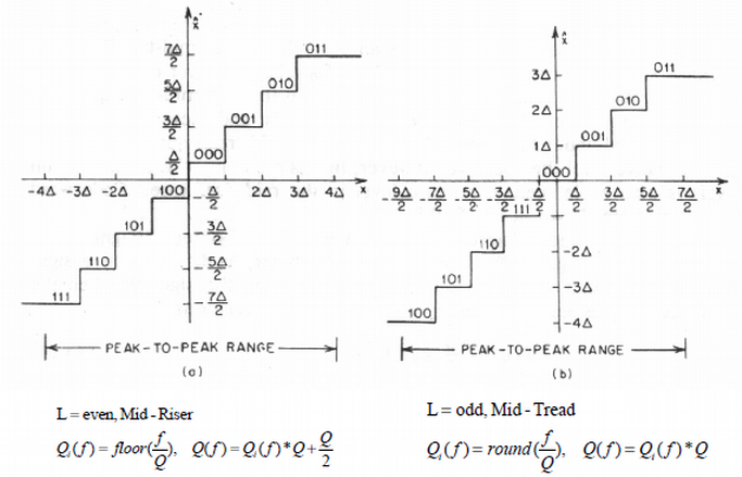
# Depending on if the quantizer has the input voltage 0 at the center of a quantization interval or on the boundary of that interval, we call the quantizer a mid-tread or a mid rise quantiser, as illustrated in the following picture:
#
#
#
# (From:http://eeweb.poly.edu/~yao/EE3414/quantization.pdf)
#
#
# Here, $Q_i(f)$ is the index after quantization (which is then encoded and sent to the receiver), and Q(f) is the de-quantization, which produces the quantized reconstructed value at the receiver.
#
# This makes mainly a difference at **very small input values**. For the mid-rise quantiser, very small values are always quantized to +/- half the quantization interval ($\pm \Delta/2$ ), whereas for the mid-tread quantizer, very small input values are always rounded to zero. You can also think about the **mid-rise** quantizer as **not having a zero** as a reconstruction value, but only very small positive and negative values.
#
# So the mid-rise can be seen as more accurate, because it also reacts to very small input values, and the mid tread can be seen as saving bit-rate because it always quantizes very small values to zero.
#
# Observe that the expectation of the quantization error power for large signals stays the same for both types.
# **Observe:** the Mid-Tread quantizer “swallows” small signal levels, since they are all rounded to zero.
# The Mid-Rise quantizer still captures small levels, but distorted.
# #### Python Example
# In[10]:
get_ipython().run_cell_magic('html', '', '\n')
# In[11]:
# Imports
import numpy as np
import matplotlib.pyplot as plt
import plotly.offline
import plotly.tools as tls
import plotly.plotly as py
# Configurations
plotly.offline.init_notebook_mode(connected=True)
import warnings; warnings.simplefilter('ignore')
# In[12]:
# Signal Processing Parameters
Fs = 32000 # Sampling frequency
T=1/Fs # Sampling Time
# In[13]:
# Input Signal
A=1
freq=500
n_period=1
period=np.round((1/freq)*n_period*Fs).astype(int)
t = np.arange(Fs+1)*T # Time vector
sinewave = A*np.sin(2*np.pi*freq*t)
# In[14]:
# Quantization and De-quantization
N=4
stepsize=(1.0-(-1.0))/(2**N)
#Encode
sinewave_quant_rise_ind=np.floor(sinewave/stepsize)
sinewave_quant_tread_ind=np.round(sinewave/stepsize)
#Decode
sinewave_quant_rise_rec=sinewave_quant_rise_ind*stepsize+stepsize/2
sinewave_quant_tread_rec=sinewave_quant_tread_ind*stepsize
# In[15]:
# Shape for plotting
t_quant=np.delete(np.repeat(t[:period+1],2),-1)
sinewave_quant_rise_rec_plot=np.delete(np.repeat(sinewave_quant_rise_rec[:period+1],2),0)
sinewave_quant_tread_rec_plot=np.delete(np.repeat(sinewave_quant_tread_rec[:period+1],2),0)
# In[16]:
# Quantization Error
quant_error_tread=sinewave_quant_tread_rec-sinewave
quant_error_rise=sinewave_quant_rise_rec-sinewave
# In[17]:
#plot
if inColab:
enable_plotly_in_cell()
fig = plt.figure(figsize=(12,8))
plt.subplot(2,1,1)
plt.plot(t[:period+1],sinewave[:period+1], label='Original Signal')
plt.plot(t_quant,sinewave_quant_rise_rec_plot, label='Quantized Signal (Mid-Rise)')
plt.plot(t_quant,sinewave_quant_tread_rec_plot, label='Quantized Signal (Mid-Tread)')
plt.title('Orignal and Quantized Signals', fontsize=18)
plt.xlabel('Time [s]')
plt.ylabel('Amplitude')
plt.yticks(np.arange(-1-stepsize, 1+stepsize, stepsize))
#plt.legend()
plt.grid()
#plt.tight_layout()
plt.subplot(2,1,2)
plt.plot(t[:period+1],quant_error_tread[:period+1], label='Quantization Error')
plt.grid()
plt.title('Quantization Error (Mid-Tread)', fontsize=18)
plt.xlabel('Time [s]')
plt.ylabel('Amplitude')
#plt.tight_layout()
plt.subplots_adjust(hspace=0.5)
plotly_fig = tls.mpl_to_plotly(fig)
plotly_fig.layout.update(showlegend=True)
plotly.offline.iplot(plotly_fig)
# In[18]:
# Listen to Audio
import IPython.display as ipd
print('Orignal Signal')
ipd.display(ipd.Audio(sinewave, rate=Fs))
print('Quantized Signal (Mid-Tread)')
ipd.display(ipd.Audio(sinewave_quant_tread_rec, rate=Fs))
print('Quantized Signal (Mid-Rise)')
ipd.display(ipd.Audio(sinewave_quant_rise_rec, rate=Fs))
print('Quantization Error (Mid-Tread)')
ipd.display(ipd.Audio(quant_error_tread, rate=Fs))
print('Quantization Error (Mid-Rise)')
ipd.display(ipd.Audio(quant_error_rise, rate=Fs))
# In[19]:
# Imports
from scipy.fftpack import fft
import plotly.offline
import plotly.tools as tls
import plotly.plotly as py
# Configurations
if inColab==False:
plotly.offline.init_notebook_mode(connected=True)
else:
enable_plotly_in_cell()
import warnings; warnings.simplefilter('ignore')
# Signal Processing Parameters
NFFT=2**10
#Frequency Analysis
freqs = np.fft.fftfreq(NFFT, d=T) # Frequency bins
original_fft=fft(sinewave, n=NFFT)
original_fft/=np.abs(original_fft).max()
quantized_tread_fft=fft(sinewave_quant_tread_rec, n=NFFT)
quantized_tread_fft/=np.abs(quantized_tread_fft).max()
quantized_rise_fft=fft(sinewave_quant_rise_rec, n=NFFT)
quantized_rise_fft/=np.abs(quantized_rise_fft).max()
# Plot
fig=plt.figure(figsize=(12,8))
plt.plot(freqs[0:NFFT//2],20*np.log10(np.abs(quantized_rise_fft[0:NFFT//2]).clip(min=1e-5)), label='Quantized Mid-Rise')
plt.plot(freqs[0:NFFT//2],20*np.log10(np.abs(quantized_tread_fft[0:NFFT//2]).clip(min=1e-5)), label='Quantized Mid-Tread')
plt.plot(freqs[0:NFFT//2],20*np.log10(np.abs(original_fft[0:NFFT//2]).clip(min=1e-5)), label='Original')
plt.grid()
plt.title('Original vs. Quantized Signal Spectrum')
plt.ylabel('Magnitude Normalized')
plt.xlabel('Frequency [Hz]')
#plt.legend()
plotly_fig = tls.mpl_to_plotly(fig)
plotly_fig.layout.update(showlegend=True)
plotly.offline.iplot(plotly_fig)
# ## Real-time Audio Python Example
#
# **Real-Time Audio Examples will not work in remote environments such as Binder and Google Colab**
# In[ ]:
get_ipython().run_cell_magic('html', '', '\n')
# In[ ]:
"""
PyAudio Example: Make a quantization between input and output
(i.e., record a few samples, quatize them with a mid-tread or
mid-rise quantizer, and play them back immediately).
Using block-wise processing instead of a for loop
Gerald Schuller, Octtober 2014
Modified to Jupyter Notebook by Renato Profeta, October 2019
"""
# Imports
import pyaudio
import struct
import numpy as np
from ipywidgets import ToggleButton, Dropdown, Button, BoundedIntText, Label
from ipywidgets import HBox, interact
import threading
# Parameters
CHUNK = 5000 #Blocksize
FORMAT = pyaudio.paInt16 #conversion format for PyAudio stream
CHANNELS = 1
RATE = 32000 #Sampling Rate in Hz
# Quantization Bit-Depth
N=8
quant_type='Mid-Tread'
# Quantization Application
def quantization_example(toggle_run):
global N, quant_type
while(True):
if toggle_run.value==True:
break
#Reading from audio input stream into data with block length "CHUNK":
data_stream = stream.read(CHUNK)
#Convert from stream of bytes to a list of short integers
#(2 bytes here) in "samples":
shorts = (struct.unpack( 'h' * CHUNK, data_stream ));
samples=np.array(list(shorts),dtype=float);
#start block-wise signal processing:
q=int((2**15-(-2**15))/(2**N))
if quant_type=='Mid-Tread':
#Mid Tread quantization:
indices=np.round(samples/q)
#de-quantization:
samples=indices*q
else:
#Mid -Rise quantizer:
indices=np.floor(samples/q)
#de-quantization:
samples=(indices*q+q/2).astype(int)
#end signal processing
#converting from short integers to a stream of bytes in "data":
#play out samples:
samples=np.clip(samples, -2**15,2**15)
samples=samples.astype(int)
data=struct.pack('h' * len(samples), *samples);
#Writing data back to audio output stream:
stream.write(data, CHUNK)
# GUI
toggle_run = ToggleButton(description='Stop')
button_start = Button(description='Start')
dropdown_type = Dropdown(
options=['Mid-Tread', 'Mid-Rise'],
value='Mid-Tread',
description='Quantization Type:',
disabled=False,
)
bitdepth_int = BoundedIntText(
value=8,
min=2,
max=16,
step=1,
description='Bit-Depth:',
disabled=False
)
q=int((2**15-(-2**15))/(2**N))
stepsize_label = Label(value="Stepsize: {:d}".format(q))
def start_button(button_start):
thread.start()
button_start.disabled=True
button_start.on_click(start_button)
def on_click_toggle_run(change):
if change['new']==False:
stream.stop_stream()
stream.close()
p.terminate()
plt.close()
toggle_run.observe(on_click_toggle_run, 'value')
def inttext_bitdepth_changed(bitdepth_int):
global N, q
if bitdepth_int['new']:
N=bitdepth_int['new']
stepsize_label.value="Stepsize: {:d}".format(int((2**15-(-2**15))/(2**N)))
bitdepth_int.observe(inttext_bitdepth_changed, names='value')
def dropdown_type_changed(dropdown_type):
global quant_type
if dropdown_type['new']:
quant_type=dropdown_type['new']
dropdown_type.observe(dropdown_type_changed, names='value')
box_buttons = HBox([button_start,toggle_run])
box_controls = HBox([bitdepth_int, dropdown_type,stepsize_label])
# Create a Thread for run_spectrogram function
thread = threading.Thread(target=quantization_example, args=(toggle_run,))
# Start Audio Stream
# Create
p = pyaudio.PyAudio()
stream = p.open(format=FORMAT,
channels=CHANNELS,
rate=RATE,
input=True,
output=True,
frames_per_buffer=CHUNK)
input_data = stream.read(CHUNK)
samples = np.frombuffer(input_data,np.int16)
display(box_buttons)
display(box_controls)
# In[ ]: