
Introduction to Pandas
April 3rd, 2015
Joris Van den Bossche
Source: https://github.com/jorisvandenbossche/2015-PyDataParisAbout me: Joris Van den Bossche
- PhD student at Ghent University and VITO, Belgium
- bio-science engineer, air quality research
- pandas core dev
->
Licensed under CC BY 4.0 Creative Commons
Content of this talk
- Why do you need pandas?
- Basic introduction to the data structures
- Guided tour through some of the pandas features with a case study about air quality
If you want to follow along, this is a notebook that you can view or run yourself:
- All materials (notebook, data, link to nbviewer): https://github.com/jorisvandenbossche/2015-PyDataParis
- You need
pandas> 0.15 (easy solution is using Anaconda)
Some imports:
%matplotlib inline
import pandas as pd
import numpy as np
import matplotlib.pyplot as plt
import seaborn

pd.options.display.max_rows = 8
Let's start with a showcase
Case study: air quality in Europe
AirBase (The European Air quality dataBase): hourly measurements of all air quality monitoring stations from Europe
Starting from these hourly data for different stations:
import airbase
data = airbase.load_data()
data
| BETR801 | BETN029 | FR04037 | FR04012 | |
|---|---|---|---|---|
| 1990-01-01 00:00:00 | NaN | 16.0 | NaN | NaN |
| 1990-01-01 01:00:00 | NaN | 18.0 | NaN | NaN |
| 1990-01-01 02:00:00 | NaN | 21.0 | NaN | NaN |
| 1990-01-01 03:00:00 | NaN | 26.0 | NaN | NaN |
| ... | ... | ... | ... | ... |
| 2012-12-31 20:00:00 | 16.5 | 2.0 | 16 | 47 |
| 2012-12-31 21:00:00 | 14.5 | 2.5 | 13 | 43 |
| 2012-12-31 22:00:00 | 16.5 | 3.5 | 14 | 42 |
| 2012-12-31 23:00:00 | 15.0 | 3.0 | 13 | 49 |
198895 rows × 4 columns
to answering questions about this data in a few lines of code:
Does the air pollution show a decreasing trend over the years?
data['1999':].resample('A').plot(ylim=[0,100])
<matplotlib.axes._subplots.AxesSubplot at 0xab4c292c>

How many exceedances of the limit values?
exceedances = data > 200
exceedances = exceedances.groupby(exceedances.index.year).sum()
ax = exceedances.loc[2005:].plot(kind='bar')
ax.axhline(18, color='k', linestyle='--')
<matplotlib.lines.Line2D at 0xab02004c>

What is the difference in diurnal profile between weekdays and weekend?
data['weekday'] = data.index.weekday
data['weekend'] = data['weekday'].isin([5, 6])
data_weekend = data.groupby(['weekend', data.index.hour])['FR04012'].mean().unstack(level=0)
data_weekend.plot()
<matplotlib.axes._subplots.AxesSubplot at 0xab3cb5cc>

We will come back to these example, and build them up step by step.
Why do you need pandas?
Why do you need pandas?
When working with tabular or structured data (like R dataframe, SQL table, Excel spreadsheet, ...):
- Import data
- Clean up messy data
- Explore data, gain insight into data
- Process and prepare your data for analysis
- Analyse your data (together with scikit-learn, statsmodels, ...)
Pandas: data analysis in python
For data-intensive work in Python the Pandas library has become essential.
What is pandas?
- Pandas can be thought of as NumPy arrays with labels for rows and columns, and better support for heterogeneous data types, but it's also much, much more than that.
- Pandas can also be thought of as
R'sdata.framein Python. - Powerful for working with missing data, working with time series data, for reading and writing your data, for reshaping, grouping, merging your data, ...
It's documentation: http://pandas.pydata.org/pandas-docs/stable/
Key features
- Fast, easy and flexible input/output for a lot of different data formats
- Working with missing data (
.dropna(),pd.isnull()) - Merging and joining (
concat,join) - Grouping:
groupbyfunctionality - Reshaping (
stack,pivot) - Powerful time series manipulation (resampling, timezones, ..)
- Easy plotting
Basic data structures
Pandas does this through two fundamental object types, both built upon NumPy arrays: the Series object, and the DataFrame object.
Series
A Series is a basic holder for one-dimensional labeled data. It can be created much as a NumPy array is created:
s = pd.Series([0.1, 0.2, 0.3, 0.4])
s
0    0.1
1    0.2
2    0.3
3    0.4
dtype: float64
Attributes of a Series: index and values
The series has a built-in concept of an index, which by default is the numbers 0 through N - 1
s.index
Int64Index([0, 1, 2, 3], dtype='int64')
You can access the underlying numpy array representation with the .values attribute:
s.values
array([ 0.1, 0.2, 0.3, 0.4])
We can access series values via the index, just like for NumPy arrays:
s[0]
0.10000000000000001
Unlike the NumPy array, though, this index can be something other than integers:
s2 = pd.Series(np.arange(4), index=['a', 'b', 'c', 'd'])
s2
a    0
b    1
c    2
d    3
dtype: int32
s2['c']
2
In this way, a Series object can be thought of as similar to an ordered dictionary mapping one typed value to another typed value:
population = pd.Series({'Germany': 81.3, 'Belgium': 11.3, 'France': 64.3, 'United Kingdom': 64.9, 'Netherlands': 16.9})
population
Belgium           11.3
France            64.3
Germany           81.3
Netherlands       16.9
United Kingdom    64.9
dtype: float64
population['France']
64.299999999999997
but with the power of numpy arrays:
population * 1000
Belgium           11300
France            64300
Germany           81300
Netherlands       16900
United Kingdom    64900
dtype: float64
We can index or slice the populations as expected:
population['Belgium']
11.300000000000001
population['Belgium':'Germany']
Belgium    11.3
France     64.3
Germany    81.3
dtype: float64
Many things you can do with numpy arrays, can also be applied on objects.
Fancy indexing, like indexing with a list or boolean indexing:
population[['France', 'Netherlands']]
France         64.3
Netherlands    16.9
dtype: float64
population[population > 20]
France            64.3
Germany           81.3
United Kingdom    64.9
dtype: float64
Element-wise operations:
population / 100
Belgium           0.113
France            0.643
Germany           0.813
Netherlands       0.169
United Kingdom    0.649
dtype: float64
A range of methods:
population.mean()
47.739999999999995
Alignment!
Only, pay attention to alignment: operations between series will align on the index:
s1 = population[['Belgium', 'France']]
s2 = population[['France', 'Germany']]
s1
Belgium    11.3
France     64.3
dtype: float64
s2
France     64.3
Germany    81.3
dtype: float64
s1 + s2
Belgium      NaN
France     128.6
Germany      NaN
dtype: float64
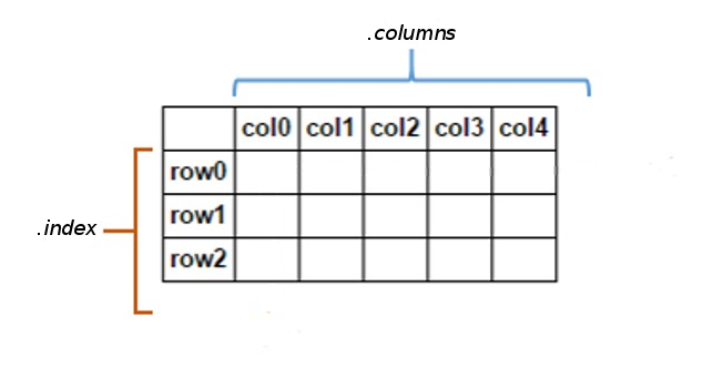
DataFrames: Multi-dimensional Data
A DataFrame is a tablular data structure (multi-dimensional object to hold labeled data) comprised of rows and columns, akin to a spreadsheet, database table, or R's data.frame object. You can think of it as multiple Series object which share the same index.
One of the most common ways of creating a dataframe is from a dictionary of arrays or lists.
Note that in the IPython notebook, the dataframe will display in a rich HTML view:
data = {'country': ['Belgium', 'France', 'Germany', 'Netherlands', 'United Kingdom'],
        'population': [11.3, 64.3, 81.3, 16.9, 64.9],
        'area': [30510, 671308, 357050, 41526, 244820],
        'capital': ['Brussels', 'Paris', 'Berlin', 'Amsterdam', 'London']}
countries = pd.DataFrame(data)
countries
| area | capital | country | population | |
|---|---|---|---|---|
| 0 | 30510 | Brussels | Belgium | 11.3 |
| 1 | 671308 | Paris | France | 64.3 |
| 2 | 357050 | Berlin | Germany | 81.3 |
| 3 | 41526 | Amsterdam | Netherlands | 16.9 |
| 4 | 244820 | London | United Kingdom | 64.9 |
Attributes of the DataFrame
A DataFrame has besides a index attribute, also a columns attribute:
countries.index
Int64Index([0, 1, 2, 3, 4], dtype='int64')
countries.columns
Index([u'area', u'capital', u'country', u'population'], dtype='object')
To check the data types of the different columns:
countries.dtypes
area            int64
capital        object
country        object
population    float64
dtype: object
An overview of that information can be given with the info() method:
countries.info()
<class 'pandas.core.frame.DataFrame'>
Int64Index: 5 entries, 0 to 4
Data columns (total 4 columns):
area          5 non-null int64
capital       5 non-null object
country       5 non-null object
population    5 non-null float64
dtypes: float64(1), int64(1), object(2)
memory usage: 160.0+ bytes
Also a DataFrame has a values attribute, but attention: when you have heterogeneous data, all values will be upcasted:
countries.values
array([[30510L, 'Brussels', 'Belgium', 11.3],
       [671308L, 'Paris', 'France', 64.3],
       [357050L, 'Berlin', 'Germany', 81.3],
       [41526L, 'Amsterdam', 'Netherlands', 16.9],
       [244820L, 'London', 'United Kingdom', 64.9]], dtype=object)
If we don't like what the index looks like, we can reset it and set one of our columns:
countries = countries.set_index('country')
countries
| area | capital | population | |
|---|---|---|---|
| country | |||
| Belgium | 30510 | Brussels | 11.3 |
| France | 671308 | Paris | 64.3 |
| Germany | 357050 | Berlin | 81.3 |
| Netherlands | 41526 | Amsterdam | 16.9 |
| United Kingdom | 244820 | London | 64.9 |
To access a Series representing a column in the data, use typical indexing syntax:
countries['area']
country
Belgium            30510
France            671308
Germany           357050
Netherlands        41526
United Kingdom    244820
Name: area, dtype: int64
As you play around with DataFrames, you'll notice that many operations which work on NumPy arrays will also work on dataframes.
Let's compute density of each country:
countries['population']*1000000 / countries['area']
country
Belgium           370.370370
France             95.783158
Germany           227.699202
Netherlands       406.973944
United Kingdom    265.092721
dtype: float64
Adding a new column to the dataframe is very simple:
countries['density'] = countries['population']*1000000 / countries['area']
countries
| area | capital | population | density | |
|---|---|---|---|---|
| country | ||||
| Belgium | 30510 | Brussels | 11.3 | 370.370370 |
| France | 671308 | Paris | 64.3 | 95.783158 |
| Germany | 357050 | Berlin | 81.3 | 227.699202 |
| Netherlands | 41526 | Amsterdam | 16.9 | 406.973944 |
| United Kingdom | 244820 | London | 64.9 | 265.092721 |
We can use masking to select certain data:
countries[countries['density'] > 300]
| area | capital | population | density | |
|---|---|---|---|---|
| country | ||||
| Belgium | 30510 | Brussels | 11.3 | 370.370370 |
| Netherlands | 41526 | Amsterdam | 16.9 | 406.973944 |
And we can do things like sorting the items in the array, and indexing to take the first two rows:
countries.sort_index(by='density', ascending=False)
| area | capital | population | density | |
|---|---|---|---|---|
| country | ||||
| Netherlands | 41526 | Amsterdam | 16.9 | 406.973944 |
| Belgium | 30510 | Brussels | 11.3 | 370.370370 |
| United Kingdom | 244820 | London | 64.9 | 265.092721 |
| Germany | 357050 | Berlin | 81.3 | 227.699202 |
| France | 671308 | Paris | 64.3 | 95.783158 |
One useful method to use is the describe method, which computes summary statistics for each column:
countries.describe()
| area | population | density | |
|---|---|---|---|
| count | 5.000000 | 5.000000 | 5.000000 |
| mean | 269042.800000 | 47.740000 | 273.183879 |
| std | 264012.827994 | 31.519645 | 123.440607 |
| min | 30510.000000 | 11.300000 | 95.783158 |
| 25% | 41526.000000 | 16.900000 | 227.699202 |
| 50% | 244820.000000 | 64.300000 | 265.092721 |
| 75% | 357050.000000 | 64.900000 | 370.370370 |
| max | 671308.000000 | 81.300000 | 406.973944 |
The plot method can be used to quickly visualize the data in different ways:
countries.plot()
<matplotlib.axes._subplots.AxesSubplot at 0xab20740c>

However, for this dataset, it does not say that much.
countries['population'].plot(kind='bar')
<matplotlib.axes._subplots.AxesSubplot at 0xab258d8c>

countries.plot(kind='scatter', x='population', y='area')
<matplotlib.axes._subplots.AxesSubplot at 0xab12eaec>

The available plotting types: ‘line’ (default), ‘bar’, ‘barh’, ‘hist’, ‘box’ , ‘kde’, ‘area’, ‘pie’, ‘scatter’, ‘hexbin’.
countries = countries.drop(['density'], axis=1)
Some notes on selecting data
One of pandas' basic features is the labeling of rows and columns, but this makes indexing also a bit more complex compared to numpy. We now have to distuinguish between:
- selection by label
- selection by position.
For a DataFrame, basic indexing selects the columns.
Selecting a single column:
countries['area']
country
Belgium            30510
France            671308
Germany           357050
Netherlands        41526
United Kingdom    244820
Name: area, dtype: int64
or multiple columns:
countries[['area', 'density']]
| area | density | |
|---|---|---|
| country | ||
| Belgium | 30510 | 370.370370 |
| France | 671308 | 95.783158 |
| Germany | 357050 | 227.699202 |
| Netherlands | 41526 | 406.973944 |
| United Kingdom | 244820 | 265.092721 |
But, slicing accesses the rows:
countries['France':'Netherlands']
| area | capital | population | density | |
|---|---|---|---|---|
| country | ||||
| France | 671308 | Paris | 64.3 | 95.783158 |
| Germany | 357050 | Berlin | 81.3 | 227.699202 |
| Netherlands | 41526 | Amsterdam | 16.9 | 406.973944 |
For more advanced indexing, you have some extra attributes:
loc: selection by labeliloc: selection by position
countries.loc['Germany', 'area']
357050
countries.loc['France':'Germany', :]
| area | capital | population | density | |
|---|---|---|---|---|
| country | ||||
| France | 671308 | Paris | 64.3 | 95.783158 |
| Germany | 357050 | Berlin | 81.3 | 227.699202 |
countries.loc[countries['density']>300, ['capital', 'population']]
| capital | population | |
|---|---|---|
| country | ||
| Belgium | Brussels | 11.3 |
| Netherlands | Amsterdam | 16.9 |
Selecting by position with iloc works similar as indexing numpy arrays:
countries.iloc[0:2,1:3]
| capital | population | |
|---|---|---|
| country | ||
| Belgium | Brussels | 11.3 |
| France | Paris | 64.3 |
The different indexing methods can also be used to assign data:
countries.loc['Belgium':'Germany', 'population'] = 10
countries
There are many, many more interesting operations that can be done on Series and DataFrame objects, but rather than continue using this toy data, we'll instead move to a real-world example, and illustrate some of the advanced concepts along the way.
Case study: air quality data of European monitoring stations (AirBase)
AirBase (The European Air quality dataBase)
AirBase: hourly measurements of all air quality monitoring stations from Europe.
from IPython.display import HTML
HTML('<iframe src=http://www.eea.europa.eu/data-and-maps/data/airbase-the-european-air-quality-database-8#tab-data-by-country width=700 height=350></iframe>')
Importing and cleaning the data
Importing and exporting data with pandas
A wide range of input/output formats are natively supported by pandas:
- CSV, text
- SQL database
- Excel
- HDF5
- json
- html
- pickle
- ...
pd.read
countries.to
Now for our case study
I downloaded some of the raw data files of AirBase and included it in the repo:
station code: BETR801, pollutant code: 8 (nitrogen dioxide)
!head -1 ./data/BETR8010000800100hour.1-1-1990.31-12-2012
Just reading the tab-delimited data:
data = pd.read_csv("data/BETR8010000800100hour.1-1-1990.31-12-2012", sep='\t')
data.head()
| 1990-01-01 | -999.000 | 0 | -999.000.1 | 0.1 | -999.000.2 | 0.2 | -999.000.3 | 0.3 | -999.000.4 | ... | -999.000.19 | 0.19 | -999.000.20 | 0.20 | -999.000.21 | 0.21 | -999.000.22 | 0.22 | -999.000.23 | 0.23 | |
|---|---|---|---|---|---|---|---|---|---|---|---|---|---|---|---|---|---|---|---|---|---|
| 0 | 1990-01-02 | -999 | 0 | -999 | 0 | -999 | 0 | -999 | 0 | -999 | ... | 57 | 1 | 58 | 1 | 54 | 1 | 49 | 1 | 48 | 1 |
| 1 | 1990-01-03 | 51 | 1 | 50 | 1 | 47 | 1 | 48 | 1 | 51 | ... | 84 | 1 | 75 | 1 | -999 | 0 | -999 | 0 | -999 | 0 |
| 2 | 1990-01-04 | -999 | 0 | -999 | 0 | -999 | 0 | -999 | 0 | -999 | ... | 69 | 1 | 65 | 1 | 64 | 1 | 60 | 1 | 59 | 1 |
| 3 | 1990-01-05 | 51 | 1 | 51 | 1 | 48 | 1 | 50 | 1 | 51 | ... | -999 | 0 | -999 | 0 | -999 | 0 | -999 | 0 | -999 | 0 |
| 4 | 1990-01-06 | -999 | 0 | -999 | 0 | -999 | 0 | -999 | 0 | -999 | ... | -999 | 0 | -999 | 0 | -999 | 0 | -999 | 0 | -999 | 0 |
5 rows × 49 columns
Not really what we want.
With using some more options of read_csv:
colnames = ['date'] + [item for pair in zip(["{:02d}".format(i) for i in range(24)], ['flag']*24) for item in pair]

data = pd.read_csv("data/BETR8010000800100hour.1-1-1990.31-12-2012",
                   sep='\t', header=None, na_values=[-999, -9999], names=colnames)
data.head()
| date | 00 | flag | 01 | flag | 02 | flag | 03 | flag | 04 | ... | 19 | flag | 20 | flag | 21 | flag | 22 | flag | 23 | flag | |
|---|---|---|---|---|---|---|---|---|---|---|---|---|---|---|---|---|---|---|---|---|---|
| 0 | 1990-01-01 | NaN | 0 | NaN | 0 | NaN | 0 | NaN | 0 | NaN | ... | NaN | 0 | NaN | 0 | NaN | 0 | NaN | 0 | NaN | 0 |
| 1 | 1990-01-02 | NaN | 1 | NaN | 1 | NaN | 1 | NaN | 1 | NaN | ... | 57 | 1 | 58 | 1 | 54 | 1 | 49 | 1 | 48 | 1 |
| 2 | 1990-01-03 | 51 | 0 | 50 | 0 | 47 | 0 | 48 | 0 | 51 | ... | 84 | 0 | 75 | 0 | NaN | 0 | NaN | 0 | NaN | 0 |
| 3 | 1990-01-04 | NaN | 1 | NaN | 1 | NaN | 1 | NaN | 1 | NaN | ... | 69 | 1 | 65 | 1 | 64 | 1 | 60 | 1 | 59 | 1 |
| 4 | 1990-01-05 | 51 | 0 | 51 | 0 | 48 | 0 | 50 | 0 | 51 | ... | NaN | 0 | NaN | 0 | NaN | 0 | NaN | 0 | NaN | 0 |
5 rows × 49 columns
So what did we do:
- specify that the values of -999 and -9999 should be regarded as NaN
- specified are own column names
For now, we disregard the 'flag' columns
data = data.drop('flag', axis=1)
data
| date | 00 | 01 | 02 | 03 | 04 | 05 | 06 | 07 | 08 | ... | 14 | 15 | 16 | 17 | 18 | 19 | 20 | 21 | 22 | 23 | |
|---|---|---|---|---|---|---|---|---|---|---|---|---|---|---|---|---|---|---|---|---|---|
| 0 | 1990-01-01 | NaN | NaN | NaN | NaN | NaN | NaN | NaN | NaN | NaN | ... | NaN | NaN | NaN | NaN | NaN | NaN | NaN | NaN | NaN | NaN |
| 1 | 1990-01-02 | NaN | NaN | NaN | NaN | NaN | NaN | NaN | NaN | NaN | ... | 55.0 | 59.0 | 58 | 59.0 | 58.0 | 57.0 | 58.0 | 54.0 | 49.0 | 48.0 |
| 2 | 1990-01-03 | 51.0 | 50.0 | 47.0 | 48.0 | 51.0 | 52.0 | 58.0 | 57.0 | NaN | ... | 69.0 | 74.0 | NaN | NaN | 103.0 | 84.0 | 75.0 | NaN | NaN | NaN |
| 3 | 1990-01-04 | NaN | NaN | NaN | NaN | NaN | NaN | NaN | NaN | NaN | ... | NaN | 71.0 | 74 | 70.0 | 70.0 | 69.0 | 65.0 | 64.0 | 60.0 | 59.0 |
| ... | ... | ... | ... | ... | ... | ... | ... | ... | ... | ... | ... | ... | ... | ... | ... | ... | ... | ... | ... | ... | ... |
| 8388 | 2012-12-28 | 26.5 | 28.5 | 35.5 | 32.0 | 35.5 | 50.5 | 62.5 | 74.5 | 76.0 | ... | 56.5 | 52.0 | 55 | 53.5 | 49.0 | 46.5 | 42.5 | 38.5 | 30.5 | 26.5 |
| 8389 | 2012-12-29 | 21.5 | 16.5 | 13.0 | 13.0 | 16.0 | 23.5 | 23.5 | 27.5 | 46.0 | ... | 48.0 | 41.5 | 36 | 33.0 | 25.5 | 21.0 | 22.0 | 20.5 | 20.0 | 15.0 |
| 8390 | 2012-12-30 | 11.5 | 9.5 | 7.5 | 7.5 | 10.0 | 11.0 | 13.5 | 13.5 | 17.5 | ... | NaN | 25.0 | 25 | 25.5 | 24.5 | 25.0 | 18.5 | 17.0 | 15.5 | 12.5 |
| 8391 | 2012-12-31 | 9.5 | 8.5 | 8.5 | 8.5 | 10.5 | 15.5 | 18.0 | 23.0 | 25.0 | ... | NaN | NaN | 28 | 27.5 | 26.0 | 21.0 | 16.5 | 14.5 | 16.5 | 15.0 |
8392 rows × 25 columns
Now, we want to reshape it: our goal is to have the different hours as row indices, merged with the date into a datetime-index.
Intermezzo: reshaping your data with stack, unstack and pivot
The docs say:
Pivot a level of the (possibly hierarchical) column labels, returning a
DataFrame (or Series in the case of an object with a single level of column labels) having a hierarchical index with a new inner-most level of row labels.

df = pd.DataFrame({'A':['one', 'one', 'two', 'two'], 'B':['a', 'b', 'a', 'b'], 'C':range(4)})
df
| A | B | C | |
|---|---|---|---|
| 0 | one | a | 0 |
| 1 | one | b | 1 |
| 2 | two | a | 2 |
| 3 | two | b | 3 |
To use stack/unstack, we need the values we want to shift from rows to columns or the other way around as the index:
df = df.set_index(['A', 'B'])
df
| C | ||
|---|---|---|
| A | B | |
| one | a | 0 |
| b | 1 | |
| two | a | 2 |
| b | 3 |
result = df['C'].unstack()
result
| B | a | b |
|---|---|---|
| A | ||
| one | 0 | 1 |
| two | 2 | 3 |
df = result.stack().reset_index(name='C')
df
| A | B | C | |
|---|---|---|---|
| 0 | one | a | 0 |
| 1 | one | b | 1 |
| 2 | two | a | 2 |
| 3 | two | b | 3 |
pivot is similar to unstack, but let you specify column names:
df.pivot(index='A', columns='B', values='C')
| B | a | b |
|---|---|---|
| A | ||
| one | 0 | 1 |
| two | 2 | 3 |
pivot_table is similar as pivot, but can work with duplicate indices and let you specify an aggregation function:
df = pd.DataFrame({'A':['one', 'one', 'two', 'two', 'one', 'two'], 'B':['a', 'b', 'a', 'b', 'a', 'b'], 'C':range(6)})
df
| A | B | C | |
|---|---|---|---|
| 0 | one | a | 0 |
| 1 | one | b | 1 |
| 2 | two | a | 2 |
| 3 | two | b | 3 |
| 4 | one | a | 4 |
| 5 | two | b | 5 |
df.pivot_table(index='A', columns='B', values='C', aggfunc='count') #'mean'
| B | a | b |
|---|---|---|
| A | ||
| one | 2 | 1 |
| two | 1 | 2 |
Back to our case study
We can now use stack to create a timeseries:
data = data.set_index('date')
data_stacked = data.stack()
data_stacked
date
1990-01-02  09    48.0
            12    48.0
            13    50.0
            14    55.0
                  ...
2012-12-31  20    16.5
            21    14.5
            22    16.5
            23    15.0
dtype: float64
Now, lets combine the two levels of the index:
data_stacked = data_stacked.reset_index(name='BETR801')
data_stacked.index = pd.to_datetime(data_stacked['date'] + data_stacked['level_1'], format="%Y-%m-%d%H")
data_stacked = data_stacked.drop(['date', 'level_1'], axis=1)
data_stacked
| BETR801 | |
|---|---|
| 1990-01-02 09:00:00 | 48.0 |
| 1990-01-02 12:00:00 | 48.0 |
| 1990-01-02 13:00:00 | 50.0 |
| 1990-01-02 14:00:00 | 55.0 |
| ... | ... |
| 2012-12-31 20:00:00 | 16.5 |
| 2012-12-31 21:00:00 | 14.5 |
| 2012-12-31 22:00:00 | 16.5 |
| 2012-12-31 23:00:00 | 15.0 |
170794 rows × 1 columns
For this talk, I put the above code in a separate function, and repeated this for some different monitoring stations:
import airbase
no2 = airbase.load_data()
- FR04037 (PARIS 13eme): urban background site at Square de Choisy
- FR04012 (Paris, Place Victor Basch): urban traffic site at Rue d'Alesia
- BETR802: urban traffic site in Antwerp, Belgium
- BETN029: rural background site in Houtem, Belgium
Exploring the data
Some useful methods:
head and tail
no2.head(3)
| BETR801 | BETN029 | FR04037 | FR04012 | |
|---|---|---|---|---|
| 1990-01-01 00:00:00 | NaN | 16 | NaN | NaN |
| 1990-01-01 01:00:00 | NaN | 18 | NaN | NaN |
| 1990-01-01 02:00:00 | NaN | 21 | NaN | NaN |
no2.tail()
| BETR801 | BETN029 | FR04037 | FR04012 | |
|---|---|---|---|---|
| 2012-12-31 19:00:00 | 21.0 | 2.5 | 28 | 67 |
| 2012-12-31 20:00:00 | 16.5 | 2.0 | 16 | 47 |
| 2012-12-31 21:00:00 | 14.5 | 2.5 | 13 | 43 |
| 2012-12-31 22:00:00 | 16.5 | 3.5 | 14 | 42 |
| 2012-12-31 23:00:00 | 15.0 | 3.0 | 13 | 49 |
info()
no2.info()
<class 'pandas.core.frame.DataFrame'>
DatetimeIndex: 198895 entries, 1990-01-01 00:00:00 to 2012-12-31 23:00:00
Data columns (total 4 columns):
BETR801    170794 non-null float64
BETN029    174807 non-null float64
FR04037    120384 non-null float64
FR04012    119448 non-null float64
dtypes: float64(4)
memory usage: 7.6 MB
Getting some basic summary statistics about the data with describe:
no2.describe()
| BETR801 | BETN029 | FR04037 | FR04012 | |
|---|---|---|---|---|
| count | 170794.000000 | 174807.000000 | 120384.000000 | 119448.000000 |
| mean | 47.914561 | 16.687756 | 40.040005 | 87.993261 |
| std | 22.230921 | 13.106549 | 23.024347 | 41.317684 |
| min | 0.000000 | 0.000000 | 0.000000 | 0.000000 |
| 25% | 32.000000 | 7.000000 | 23.000000 | 61.000000 |
| 50% | 46.000000 | 12.000000 | 37.000000 | 88.000000 |
| 75% | 61.000000 | 23.000000 | 54.000000 | 115.000000 |
| max | 339.000000 | 115.000000 | 256.000000 | 358.000000 |
Quickly visualizing the data
no2.plot(kind='box', ylim=[0,250])
<matplotlib.axes._subplots.AxesSubplot at 0xaa1d544c>

no2['BETR801'].plot(kind='hist', bins=50)
<matplotlib.axes._subplots.AxesSubplot at 0xaabe97ec>

no2.plot(figsize=(12,6))
<matplotlib.axes._subplots.AxesSubplot at 0xa7b3e74c>

This does not say too much ..
We can select part of the data (eg the latest 500 data points):
no2[-500:].plot(figsize=(12,6))
<matplotlib.axes._subplots.AxesSubplot at 0xa7c325ec>

Or we can use some more advanced time series features -> next section!
Working with time series data
When we ensure the DataFrame has a DatetimeIndex, time-series related functionality becomes available:
no2.index
<class 'pandas.tseries.index.DatetimeIndex'>
[1990-01-01 00:00:00, ..., 2012-12-31 23:00:00]
Length: 198895, Freq: None, Timezone: None
Indexing a time series works with strings:
no2["2010-01-01 09:00": "2010-01-01 12:00"]
| BETR801 | BETN029 | FR04037 | FR04012 | |
|---|---|---|---|---|
| 2010-01-01 09:00:00 | 17 | 7 | 19 | 41 |
| 2010-01-01 10:00:00 | 18 | 5 | 21 | 48 |
| 2010-01-01 11:00:00 | 17 | 4 | 23 | 63 |
| 2010-01-01 12:00:00 | 18 | 4 | 22 | 57 |
A nice feature is "partial string" indexing, where we can do implicit slicing by providing a partial datetime string.
E.g. all data of 2012:
no2['2012']
| BETR801 | BETN029 | FR04037 | FR04012 | |
|---|---|---|---|---|
| 2012-01-01 00:00:00 | 21.0 | 1.0 | 17 | 56 |
| 2012-01-01 01:00:00 | 18.0 | 1.0 | 16 | 50 |
| 2012-01-01 02:00:00 | 20.0 | 1.0 | 14 | 46 |
| 2012-01-01 03:00:00 | 16.0 | 1.0 | 17 | 47 |
| ... | ... | ... | ... | ... |
| 2012-12-31 20:00:00 | 16.5 | 2.0 | 16 | 47 |
| 2012-12-31 21:00:00 | 14.5 | 2.5 | 13 | 43 |
| 2012-12-31 22:00:00 | 16.5 | 3.5 | 14 | 42 |
| 2012-12-31 23:00:00 | 15.0 | 3.0 | 13 | 49 |
8784 rows × 4 columns
Or all data of January up to March 2012:
data['2012-01':'2012-03']
| 00 | 01 | 02 | 03 | 04 | 05 | 06 | 07 | 08 | 09 | ... | 14 | 15 | 16 | 17 | 18 | 19 | 20 | 21 | 22 | 23 | |
|---|---|---|---|---|---|---|---|---|---|---|---|---|---|---|---|---|---|---|---|---|---|
| date | |||||||||||||||||||||
| 2012-01-01 | 21 | 18 | 20.0 | 16.0 | 13 | 17.0 | 15.0 | 13.0 | 15.0 | 15.0 | ... | 31.5 | 33.5 | 32.5 | 30 | 25.0 | 20.0 | 14.0 | 13 | 15.0 | 14 |
| 2012-01-02 | NaN | NaN | 10.5 | 12.0 | 12 | 39.0 | 49.5 | 52.5 | 45.0 | 48.0 | ... | 32.0 | 38.0 | 43.0 | 61 | 56.0 | 46.0 | 39.0 | 33 | 24.0 | 20 |
| 2012-01-03 | 18 | NaN | NaN | 14.0 | 23 | 31.5 | 36.0 | 40.0 | 32.5 | 26.0 | ... | 24.0 | 28.0 | 25.0 | 28 | 25.0 | 26.0 | 22.0 | 21 | 20.0 | 19 |
| 2012-01-04 | 16 | 16 | NaN | 13.0 | 14 | 17.0 | 26.0 | 33.0 | 36.0 | 36.0 | ... | 41.0 | 42.0 | 52.5 | 48 | 39.0 | 32.5 | 23.0 | 16 | 13.0 | 12 |
| ... | ... | ... | ... | ... | ... | ... | ... | ... | ... | ... | ... | ... | ... | ... | ... | ... | ... | ... | ... | ... | ... |
| 2012-02-26 | 56 | 53 | 56.0 | 53.0 | 53 | NaN | NaN | 48.0 | 50.0 | 52.5 | ... | 25.0 | 32.0 | 37.5 | 50 | 50.0 | 44.0 | 54.5 | 54 | 54.5 | 67 |
| 2012-02-27 | 59 | 47 | 50.0 | 51.5 | 59 | 65.0 | NaN | NaN | 70.0 | 62.0 | ... | 56.0 | 61.0 | 70.0 | 68 | 60.0 | 56.0 | 54.0 | 42 | 36.0 | 28 |
| 2012-02-28 | 24 | 23 | 20.0 | 21.0 | 27 | 43.0 | 55.0 | NaN | NaN | 47.0 | ... | 49.0 | 55.0 | 61.0 | 59 | 61.0 | 53.5 | 52.0 | 52 | 50.0 | 48 |
| 2012-02-29 | 45 | 39 | 35.0 | 32.5 | 34 | 47.0 | 51.5 | 52.5 | NaN | NaN | ... | 50.0 | 56.0 | 61.0 | 67 | 73.5 | 73.0 | 72.5 | 70 | 69.0 | 62 |
60 rows × 24 columns
Time and date components can be accessed from the index:
no2.index.hour
array([ 0, 1, 2, ..., 21, 22, 23])
no2.index.year
array([1990, 1990, 1990, ..., 2012, 2012, 2012])
The power of pandas: resample
A very powerfull method is resample: converting the frequency of the time series (e.g. from hourly to daily data).
The time series has a frequency of 1 hour. I want to change this to daily:
no2.resample('D').head()
| BETR801 | BETN029 | FR04037 | FR04012 | |
|---|---|---|---|---|
| 1990-01-01 | NaN | 21.500000 | NaN | NaN |
| 1990-01-02 | 53.923077 | 35.000000 | NaN | NaN |
| 1990-01-03 | 63.000000 | 29.136364 | NaN | NaN |
| 1990-01-04 | 65.250000 | 42.681818 | NaN | NaN |
| 1990-01-05 | 63.846154 | 40.136364 | NaN | NaN |
By default, resample takes the mean as aggregation function, but other methods can also be specified:
no2.resample('D', how='max').head()
| BETR801 | BETN029 | FR04037 | FR04012 | |
|---|---|---|---|---|
| 1990-01-01 | NaN | 41 | NaN | NaN |
| 1990-01-02 | 59 | 59 | NaN | NaN |
| 1990-01-03 | 103 | 47 | NaN | NaN |
| 1990-01-04 | 74 | 58 | NaN | NaN |
| 1990-01-05 | 84 | 67 | NaN | NaN |
The string to specify the new time frequency: http://pandas.pydata.org/pandas-docs/dev/timeseries.html#offset-aliases
These strings can also be combined with numbers, eg '10D'.
Further exploring the data:
no2.resample('M').plot() # 'A'
<matplotlib.axes._subplots.AxesSubplot at 0xa96348ac>

# no2['2012'].resample('D').plot()
no2.loc['2009':, 'FR04037'].resample('M', how=['mean', 'median']).plot()
<matplotlib.axes._subplots.AxesSubplot at 0xa7bdc64c>

Question: The evolution of the yearly averages with, and the overall mean of all stations
no2_1999 = no2['1999':]
no2_1999.resample('A').plot()
no2_1999.mean(axis=1).resample('A').plot(color='k', linestyle='--', linewidth=4)
<matplotlib.axes._subplots.AxesSubplot at 0xa93b380c>

Analysing the data
Intermezzo - the groupby operation (split-apply-combine)
By "group by" we are referring to a process involving one or more of the following steps
- Splitting the data into groups based on some criteria
- Applying a function to each group independently
- Combining the results into a data structure

Similar to SQL GROUP BY
The example of the image in pandas syntax:
df = pd.DataFrame({'key':['A','B','C','A','B','C','A','B','C'],
                   'data': [0, 5, 10, 5, 10, 15, 10, 15, 20]})
df
| data | key | |
|---|---|---|
| 0 | 0 | A |
| 1 | 5 | B |
| 2 | 10 | C |
| 3 | 5 | A |
| ... | ... | ... |
| 5 | 15 | C |
| 6 | 10 | A |
| 7 | 15 | B |
| 8 | 20 | C |
9 rows × 2 columns
df.groupby('key').aggregate('sum') # np.sum
| data | |
|---|---|
| key | |
| A | 15 |
| B | 30 |
| C | 45 |
df.groupby('key').sum()
| data | |
|---|---|
| key | |
| A | 15 |
| B | 30 |
| C | 45 |
Back to the air quality data
Question: how does the typical monthly profile look like for the different stations?
First, we add a column to the dataframe that indicates the month (integer value of 1 to 12):
no2['month'] = no2.index.month
Now, we can calculate the mean of each month over the different years:
no2.groupby('month').mean()
| BETR801 | BETN029 | FR04037 | FR04012 | |
|---|---|---|---|---|
| month | ||||
| 1 | 50.927088 | 20.304075 | 47.634409 | 82.472813 |
| 2 | 54.168021 | 19.938929 | 50.564499 | 83.973207 |
| 3 | 54.598322 | 19.424205 | 47.862715 | 96.272138 |
| 4 | 51.491741 | 18.183433 | 40.943117 | 95.962862 |
| ... | ... | ... | ... | ... |
| 9 | 49.220250 | 14.605979 | 39.706019 | 93.000316 |
| 10 | 50.894911 | 17.660149 | 44.010934 | 86.297836 |
| 11 | 50.254468 | 19.372193 | 45.564683 | 87.173878 |
| 12 | 48.644117 | 21.007089 | 45.262243 | 81.817977 |
12 rows × 4 columns
no2.groupby('month').mean().plot()
<matplotlib.axes._subplots.AxesSubplot at 0xa93495cc>

Question: The typical diurnal profile for the different stations
no2.groupby(no2.index.hour).mean().plot()
<matplotlib.axes._subplots.AxesSubplot at 0xa4a46acc>

Question: What is the difference in the typical diurnal profile between week and weekend days.
no2.index.weekday?
no2['weekday'] = no2.index.weekday
Add a column indicating week/weekend
no2['weekend'] = no2['weekday'].isin([5, 6])
data_weekend = no2.groupby(['weekend', no2.index.hour]).mean()
data_weekend.head()
| BETR801 | BETN029 | FR04037 | FR04012 | month | weekday | ||
|---|---|---|---|---|---|---|---|
| weekend | |||||||
| False | 0 | 40.008066 | 17.487512 | 34.439398 | 52.094663 | 6.520355 | 1.998157 |
| 1 | 38.281875 | 17.162671 | 31.585121 | 44.721629 | 6.518121 | 1.997315 | |
| 2 | 38.601189 | 16.800076 | 30.865143 | 43.518539 | 6.520511 | 2.000000 | |
| 3 | 42.633946 | 16.591031 | 32.963500 | 51.942135 | 6.518038 | 2.002360 | |
| 4 | 49.853566 | 16.791971 | 40.780162 | 72.547472 | 6.514098 | 2.003883 |
data_weekend_FR04012 = data_weekend['FR04012'].unstack(level=0)
data_weekend_FR04012.head()
| weekend | False | True |
|---|---|---|
| 0 | 52.094663 | 69.817219 |
| 1 | 44.721629 | 60.697248 |
| 2 | 43.518539 | 54.407904 |
| 3 | 51.942135 | 53.534933 |
| 4 | 72.547472 | 57.472830 |
data_weekend_FR04012.plot()
<matplotlib.axes._subplots.AxesSubplot at 0xa95081cc>
Question: What are the number of exceedances of hourly values above the European limit 200 µg/m3 ?
exceedances = no2 > 200
# group by year and count exceedances (sum of boolean)
exceedances = exceedances.groupby(exceedances.index.year).sum()
ax = exceedances.loc[2005:].plot(kind='bar')
ax.axhline(18, color='k', linestyle='--')
<matplotlib.lines.Line2D at 0xa94c7b0c>

Question: Visualize the typical week profile for the different stations as boxplots.
Tip: the boxplot method of a DataFrame expects the data for the different boxes in different columns)
# add a weekday and week column
no2['weekday'] = no2.index.weekday
no2['week'] = no2.index.week
no2.head()
| BETR801 | BETN029 | FR04037 | FR04012 | month | weekday | weekend | week | |
|---|---|---|---|---|---|---|---|---|
| 1990-01-01 00:00:00 | NaN | 16 | NaN | NaN | 1 | 0 | False | 1 |
| 1990-01-01 01:00:00 | NaN | 18 | NaN | NaN | 1 | 0 | False | 1 |
| 1990-01-01 02:00:00 | NaN | 21 | NaN | NaN | 1 | 0 | False | 1 |
| 1990-01-01 03:00:00 | NaN | 26 | NaN | NaN | 1 | 0 | False | 1 |
| 1990-01-01 04:00:00 | NaN | 21 | NaN | NaN | 1 | 0 | False | 1 |
# pivot table so that the weekdays are the different columns
data_pivoted = no2['2012'].pivot_table(columns='weekday', index='week', values='FR04037')
data_pivoted.head()
| weekday | 0 | 1 | 2 | 3 | 4 | 5 | 6 |
|---|---|---|---|---|---|---|---|
| week | |||||||
| 1 | 24.625000 | 23.875000 | 26.208333 | 17.500000 | 40.208333 | 24.625000 | 22.375000 |
| 2 | 39.125000 | 44.125000 | 57.583333 | 50.750000 | 40.791667 | 34.750000 | 32.250000 |
| 3 | 45.208333 | 66.333333 | 51.958333 | 28.250000 | 28.291667 | 18.416667 | 18.333333 |
| 4 | 35.333333 | 49.500000 | 49.375000 | 48.916667 | 63.458333 | 34.250000 | 25.250000 |
| 5 | 47.791667 | 38.791667 | 54.333333 | 50.041667 | 51.458333 | 46.541667 | 35.458333 |
box = data_pivoted.boxplot()
/home/joris/miniconda/lib/python2.7/site-packages/pandas/tools/plotting.py:2633: FutureWarning:
The default value for 'return_type' will change to 'axes' in a future release.
 To use the future behavior now, set return_type='axes'.
 To keep the previous behavior and silence this warning, set return_type='dict'.
  warnings.warn(msg, FutureWarning)

Exercise: Calculate the correlation between the different stations
no2[['BETR801', 'BETN029', 'FR04037', 'FR04012']].corr()
| BETR801 | BETN029 | FR04037 | FR04012 | |
|---|---|---|---|---|
| BETR801 | 1.000000 | 0.464085 | 0.561676 | 0.394446 |
| BETN029 | 0.464085 | 1.000000 | 0.401864 | 0.186997 |
| FR04037 | 0.561676 | 0.401864 | 1.000000 | 0.433466 |
| FR04012 | 0.394446 | 0.186997 | 0.433466 | 1.000000 |
no2[['BETR801', 'BETN029', 'FR04037', 'FR04012']].resample('D').corr()
| BETR801 | BETN029 | FR04037 | FR04012 | |
|---|---|---|---|---|
| BETR801 | 1.000000 | 0.581701 | 0.663855 | 0.459885 |
| BETN029 | 0.581701 | 1.000000 | 0.527390 | 0.312484 |
| FR04037 | 0.663855 | 0.527390 | 1.000000 | 0.453584 |
| FR04012 | 0.459885 | 0.312484 | 0.453584 | 1.000000 |
no2 = no2[['BETR801', 'BETN029', 'FR04037', 'FR04012']]
Further reading
- the documentation: http://pandas.pydata.org/pandas-docs/stable/
- Wes McKinney's book "Python for Data Analysis"
- lots of tutorials on the internet, eg http://github.com/jvns/pandas-cookbook
What's new in pandas
Some recent enhancements of the last year (versions 0.14 to 0.16):
- Better integration for categorical data (
CategoricalandCategoricalIndex) - The same for
TimedeltaandTimedeltaIndex - More flexible SQL interface based on
sqlalchemy - MultiIndexing using slicers
.dtaccessor for accesing datetime-properties from columns- Groupby enhancements
- And a lot of enhancements and bug fixes
How can you help?
We need you!
Contributions are very welcome and can be in different domains:
- reporting issues
- improving the documentation
- testing release candidates and provide feedback
- triaging and fixing bugs
- implementing new features
- spreading the word
Thanks for listening! Questions?
Slides and data: Source: https://github.com/jorisvandenbossche/2015-PyDataParis
Slides presented with 'live reveal' https://github.com/damianavila/RISE