Analyzing NYC High School Data : Introduction¶

One of the most controversial issues in the U.S. educational system is the effectiveness of standardized tests, and whether they're unfair to certain groups or not. We will examine this in connection with the SAT.

The SAT, or Scholastic Aptitude Test, is an exam that U.S. high school students take before applying to college. Colleges take the test scores into account when deciding who to admit, so it's fairly important to perform well on it.

The test consists of three sections, each of which has 800 possible points. The combined score is out of 2,400 possible points. Organizations often rank high schools by their average SAT scores. The scores are also considered a measure of overall school district quality.

Thus from students perspective and from the point of view of schools, SAT results are very important.

Investigating the correlations between SAT scores and demographics might shed some light into the most controversial issues in the U.S. educational system, if the standard tests are unfair or not.

Objective¶

We could correlate SAT scores with factors like race, gender, income, and more to see if standardized tests are unfair to certain groups or not.

Data Sets¶

New York City makes its data on high school SAT scores available online, as well as the demographics for each high school.

Unfortunately, combining both of the data sets won't give us all of the information we want to create a bigger picture. We'll need to supplement our data with other sources to do our full analysis.

The same website has several related data sets covering demographic information and test scores.

We will be using attendance information for each school, class size, school survey and more. Complete list is given below.

Here are the links to all of the data sets we'll be using:

Student SAT scores by high school
SAT scores by school - SAT scores for each high school in New York City
School attendance - Attendance information for each school in New York City
Class size - Information on class size for each school
AP test results - Advanced Placement (AP) exam results for each high school (passing an optional AP exam in a particular subject can earn a student college credit in that subject)
Graduation outcomes - The percentage of students who graduated, and other outcome information
Demographics - Demographic information for each school
School survey - Surveys of parents, teachers, and students at each school

All of these data sets are interrelated. We'll need to combine them into a single data set before we can find correlations.

Reading the data¶

We are using two types of data. One set is in .csv format while the other is in .txt format. We will use pandas read_csv() function to read these data. Though the files in .txt needs some special attention.

Reading `.csv` files¶

In [1]:

import pandas as pd
import numpy
import re

# List of file names 

data_files = [
    "ap_2010.csv",
    "class_size.csv",
    "demographics.csv",
    "graduation.csv",
    "hs_directory.csv",
    "sat_results.csv"
]

# creating an empty list to store all the data
data = {}


# Reading the files and adding it to the data dictionary

for file in data_files:
    d = pd.read_csv("schools/{0}".format(file))
    data[file.replace(".csv", "")] = d

Reading `.txt` files¶

Due to the complexity of the format, we need to

Specify the keyword argument delimiter="\t".
Specify the keyword argument encoding="windows-1252".

In [2]:

# Reading the survey files

all_survey = pd.read_csv("schools/survey_all.txt", delimiter="\t", encoding='windows-1252')
d75_survey = pd.read_csv("schools/survey_d75.txt", delimiter="\t", encoding='windows-1252')

# Combing the two survey data into one

survey = pd.concat([all_survey, d75_survey], axis=0)

# Printing the first few lines of the survey data

survey.head()

Out[2]:

	N_p	N_s	N_t	aca_p_11	aca_s_11	aca_t_11	aca_tot_11	bn	com_p_11	com_s_11	...	t_q8c_1	t_q8c_2	t_q8c_3	t_q8c_4	t_q9	t_q9_1	t_q9_2	t_q9_3	t_q9_4	t_q9_5
0	90.0	NaN	22.0	7.8	NaN	7.9	7.9	M015	7.6	NaN	...	29.0	67.0	5.0	0.0	NaN	5.0	14.0	52.0	24.0	5.0
1	161.0	NaN	34.0	7.8	NaN	9.1	8.4	M019	7.6	NaN	...	74.0	21.0	6.0	0.0	NaN	3.0	6.0	3.0	78.0	9.0
2	367.0	NaN	42.0	8.6	NaN	7.5	8.0	M020	8.3	NaN	...	33.0	35.0	20.0	13.0	NaN	3.0	5.0	16.0	70.0	5.0
3	151.0	145.0	29.0	8.5	7.4	7.8	7.9	M034	8.2	5.9	...	21.0	45.0	28.0	7.0	NaN	0.0	18.0	32.0	39.0	11.0
4	90.0	NaN	23.0	7.9	NaN	8.1	8.0	M063	7.9	NaN	...	59.0	36.0	5.0	0.0	NaN	10.0	5.0	10.0	60.0	15.0

5 rows × 2773 columns

We can see that there are more than 2500 columns in this data set. Fortunately there is a data dictionary available for this data set.

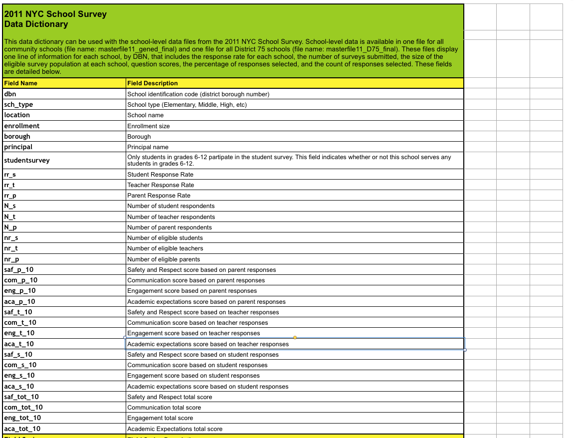
From this given list, we will take

dbn : To get the unique identification for each values

And columns from studentsurvey fields. Below you can find all the columns and its description that we will be using in this analysis.

Column	Description
dbn	School identification code (district borough number)
N_p	NUMBER OF RESPONDENTS_Parents
N_s	NUMBER OF RESPONDENTS_Students
N_t	NUMBER OF RESPONDENTS_Teachers
aca_p_11	Academic expectation score from Parent's response
aca_s_11	Academic expectation score from Student's response
aca_t_11	Academic expectation score from Teacher's response
aca_tot_11	Academic expectation score Total
com_p_11	Communication score from Parent's response
com_s_11	Communication score from Student's response
com_t_11	Communication score from Teacher's response
com_tot_11	Communication score Total
eng_p_11	Engagement score from Parent's response
eng_s_11	Engagement score from Student's response
eng_t_11	Engagement score from Teacher's response
eng_tot_11	Engagement score Total
rr_p	Resonse rate_Parents
rr_s	Resonse rate_Students
rr_t	Resonse rate_Teachers
saf_p_11	Safety and Respect score from Parent's response
saf_s_11	Safety and Respect score from Students's response
saf_t_11	Safety and Respect score from Teacher's response
saf_tot_11	Safety and Respect score Total

In order to match with the unique identification for schools in the previous data sets, we will change dbn to DBN in survey fields as well.

In [3]:

# Creating and Copying values to new DBN column
survey["DBN"] = survey["dbn"]


# Selecting the required columns
survey_fields = [
    "DBN", 
    "rr_s", 
    "rr_t", 
    "rr_p", 
    "N_s", 
    "N_t", 
    "N_p", 
    "saf_p_11", 
    "com_p_11", 
    "eng_p_11", 
    "aca_p_11", 
    "saf_t_11", 
    "com_t_11", 
    "eng_t_11", 
    "aca_t_11", 
    "saf_s_11", 
    "com_s_11", 
    "eng_s_11", 
    "aca_s_11", 
    "saf_tot_11", 
    "com_tot_11", 
    "eng_tot_11", 
    "aca_tot_11",
]

# Reassigning only the selected columns to survey data 
survey = survey.loc[:,survey_fields]

# Adding survey data to Data Dictionary
data["survey"] = survey

In [4]:

# Printing all the Keys in Data Dictionary

print("All Keys in Data Dictionary  \n-------------")
for key in data:
    print (key)
print (" \n  \n") 

# Checking if the values linked to the keys has 'DBN' column
# and Printing the keys without 'DBN' values

print("All Keys in Data Dictionary without 'DBN' column \n----------- ")

for key in data:
    if 'DBN' not in data['{}'.format(key)]:
        print(key, "DBN not present")
        
    print("\n")
    
    if 'dbn' in data['{}'.format(key)]:
        print(key, "dbn present")

All Keys in Data Dictionary  
-------------
graduation
survey
demographics
sat_results
ap_2010
hs_directory
class_size
 
  

All Keys in Data Dictionary without 'DBN' column 
----------- 










hs_directory DBN not present


hs_directory dbn present
class_size DBN not present

'DBN' columns are the unique identification for each schools in our dataset. Without having DBN column it will be difficult to work with the data.

Now that class_size, hs_directory are missing 'DBN' columns, we need to add it to them.

We can see that hs_directory has 'dbn' column present. So we just need to standardise the column name.

But for class_size we need to look further in detail.

Adding DBN columns¶

In [5]:

# Adding and Assigning a new column 'DBN' to 'hs_directory'

data["hs_directory"]["DBN"] = data["hs_directory"]["dbn"]

print(data["hs_directory"]["DBN"][:5])

# Inspecting class_size data set
data["class_size"][:5]

0    17K548
1    09X543
2    09X327
3    02M280
4    28Q680
Name: DBN, dtype: object

Out[5]:

	CSD	BOROUGH	SCHOOL CODE	SCHOOL NAME	GRADE	PROGRAM TYPE	CORE SUBJECT (MS CORE and 9-12 ONLY)	CORE COURSE (MS CORE and 9-12 ONLY)	SERVICE CATEGORY(K-9* ONLY)	NUMBER OF STUDENTS / SEATS FILLED	NUMBER OF SECTIONS	AVERAGE CLASS SIZE	SIZE OF SMALLEST CLASS	SIZE OF LARGEST CLASS	DATA SOURCE	SCHOOLWIDE PUPIL-TEACHER RATIO
0	1	M	M015	P.S. 015 Roberto Clemente	0K	GEN ED	-	-	-	19.0	1.0	19.0	19.0	19.0	ATS	NaN
1	1	M	M015	P.S. 015 Roberto Clemente	0K	CTT	-	-	-	21.0	1.0	21.0	21.0	21.0	ATS	NaN
2	1	M	M015	P.S. 015 Roberto Clemente	01	GEN ED	-	-	-	17.0	1.0	17.0	17.0	17.0	ATS	NaN
3	1	M	M015	P.S. 015 Roberto Clemente	01	CTT	-	-	-	17.0	1.0	17.0	17.0	17.0	ATS	NaN
4	1	M	M015	P.S. 015 Roberto Clemente	02	GEN ED	-	-	-	15.0	1.0	15.0	15.0	15.0	ATS	NaN

From our data dictionary we know that DBN means District Borough Number. This we can get by combining the values in CSD column and that in SCHOOL CODE.

But from out previous examples like "09X327" we know that DBN follows 2 digits of CSD followed by the school code.

From above dataframe, we can see that some of the CSD values are 1 digit. So we first need to convert into 2 digits by padding it with a preceding 0 value.

So we will first create a column called padded_csd using zfill() method and then concatanate this string with school code to create DBN column

In [6]:

# Creating a function to pad a single digit with 0 in the front
# Using zfill(width=2)

def pad_csd(num):
    return str(num).zfill(2)


# Applying the function to all values of CSD column in Class_size    
data["class_size"]["padded_csd"] = data["class_size"]["CSD"].apply(pad_csd)

# Concatanating padded csd and school code to create DBN
data["class_size"]["DBN"] = data["class_size"]["padded_csd"] + data["class_size"]["SCHOOL CODE"]


data["class_size"].head(2)

Out[6]:

	CSD	BOROUGH	SCHOOL CODE	SCHOOL NAME	GRADE	PROGRAM TYPE	CORE SUBJECT (MS CORE and 9-12 ONLY)	CORE COURSE (MS CORE and 9-12 ONLY)	SERVICE CATEGORY(K-9* ONLY)	NUMBER OF STUDENTS / SEATS FILLED	NUMBER OF SECTIONS	AVERAGE CLASS SIZE	SIZE OF SMALLEST CLASS	SIZE OF LARGEST CLASS	DATA SOURCE	SCHOOLWIDE PUPIL-TEACHER RATIO	padded_csd	DBN
0	1	M	M015	P.S. 015 Roberto Clemente	0K	GEN ED	-	-	-	19.0	1.0	19.0	19.0	19.0	ATS	NaN	01	01M015
1	1	M	M015	P.S. 015 Roberto Clemente	0K	CTT	-	-	-	21.0	1.0	21.0	21.0	21.0	ATS	NaN	01	01M015

Now that we have a uniquely identifyable column in each dataset, we can combine the datasets. But it would be great to deal with aggregation of certain columns rather than individual ones.

So let's start looking at some of the data sets.

Adding column for SAT Score¶

For our analysis, we need SAT score. So lets start with that.

In [7]:

data["sat_results"][:3]

Out[7]:

	DBN	SCHOOL NAME	Num of SAT Test Takers	SAT Critical Reading Avg. Score	SAT Math Avg. Score	SAT Writing Avg. Score
0	01M292	HENRY STREET SCHOOL FOR INTERNATIONAL STUDIES	29	355	404	363
1	01M448	UNIVERSITY NEIGHBORHOOD HIGH SCHOOL	91	383	423	366
2	01M450	EAST SIDE COMMUNITY SCHOOL	70	377	402	370

In [8]:

data["sat_results"]['SAT Critical Reading Avg. Score'][:2]

Out[8]:

0    355
1    383
Name: SAT Critical Reading Avg. Score, dtype: object

We can see that there are 3 columns namely 'SAT Math Avg. Score', 'SAT Critical Reading Avg. Score' and 'SAT Writing Avg. Score'. It would be great if we have to deal with just one column which is the total value of the three.

But from the above result we can see that the data type of these columns are 'objects'. First we need to convert them from string to numeric numbers in order to be able to add them.

Converting columns to numeric¶

We will use pd.to_numeric() function to achieve this.

In [9]:

cols = ['SAT Math Avg. Score', 'SAT Critical Reading Avg. Score', 'SAT Writing Avg. Score']

# Converting and reassigning to Numeric value
for c in cols:
    data["sat_results"][c] = pd.to_numeric(data["sat_results"][c], errors="coerce")

# Creating a new column and adding all the SAT values
data['sat_results']['sat_score'] = data['sat_results'][cols[0]] + data['sat_results'][cols[1]] + data['sat_results'][cols[2]]

data['sat_results'].head(2)

Out[9]:

	DBN	SCHOOL NAME	Num of SAT Test Takers	SAT Critical Reading Avg. Score	SAT Math Avg. Score	SAT Writing Avg. Score	sat_score
0	01M292	HENRY STREET SCHOOL FOR INTERNATIONAL STUDIES	29	355.0	404.0	363.0	1122.0
1	01M448	UNIVERSITY NEIGHBORHOOD HIGH SCHOOL	91	383.0	423.0	366.0	1172.0

Adding columns for Location Coordinates¶

Now that we have DBN and sat_Score aggregate, we can look into the location of the schools.

We'll parse the latitude and longitude coordinates for each school. This will enable us to map the schools and uncover any geographic patterns in the data.

The coordinates are currently in the text field Location 1 in the hs_directory data set.

Though we need to extract the longitude and latitude from the text file.

In [10]:

data['hs_directory']['Location 1'][0]

Out[10]:

'883 Classon Avenue\nBrooklyn, NY 11225\n(40.67029890700047, -73.96164787599963)'

In [11]:

#Creating a function to find parse latitude ie. the first part within the bracket

def find_lat(loc):
    coords = re.findall("\(.+, .+\)", loc)
    lat = coords[0].split(",")[0].replace("(", "")
    return lat


#Creating a function to find parse latitude ie. the second part within the bracket

def find_lon(loc):
    coords = re.findall("\(.+, .+\)", loc)
    lon = coords[0].split(",")[1].replace(")", "").strip()
    return lon

# Appying the functions and Creating new columns to store lat and long

data["hs_directory"]["lat"] = data["hs_directory"]["Location 1"].apply(find_lat)
data["hs_directory"]["lon"] = data["hs_directory"]["Location 1"].apply(find_lon)


# Converting the string values to numerical and reassigning 

data["hs_directory"]["lat"] = pd.to_numeric(data["hs_directory"]["lat"], errors="coerce")
data["hs_directory"]["lon"] = pd.to_numeric(data["hs_directory"]["lon"], errors="coerce")

In [12]:

data["hs_directory"].head(2)

Out[12]:

	dbn	school_name	boro	building_code	phone_number	fax_number	grade_span_min	grade_span_max	expgrade_span_min	expgrade_span_max	...	priority05	priority06	priority07	priority08	priority09	priority10	Location 1	DBN	lat	lon
0	17K548	Brooklyn School for Music & Theatre	Brooklyn	K440	718-230-6250	718-230-6262	9	12	NaN	NaN	...	NaN	NaN	NaN	NaN	NaN	NaN	883 Classon Avenue\nBrooklyn, NY 11225\n(40.67...	17K548	40.670299	-73.961648
1	09X543	High School for Violin and Dance	Bronx	X400	718-842-0687	718-589-9849	9	12	NaN	NaN	...	NaN	NaN	NaN	NaN	NaN	NaN	1110 Boston Road\nBronx, NY 10456\n(40.8276026...	09X543	40.827603	-73.904475

2 rows × 61 columns

So far we have added some important columns to individual dataframes. Now the issue we need to address is to find and remove unnecessary rows and columns in the data dictionary.

So we will be condensing our datasets.

Condense datasets¶

The first data set that we'll condense is class_size. The first few rows of class_size look like this:

In [13]:

data["class_size"].head(5)

Out[13]:

	CSD	BOROUGH	SCHOOL CODE	SCHOOL NAME	GRADE	PROGRAM TYPE	CORE SUBJECT (MS CORE and 9-12 ONLY)	CORE COURSE (MS CORE and 9-12 ONLY)	SERVICE CATEGORY(K-9* ONLY)	NUMBER OF STUDENTS / SEATS FILLED	NUMBER OF SECTIONS	AVERAGE CLASS SIZE	SIZE OF SMALLEST CLASS	SIZE OF LARGEST CLASS	DATA SOURCE	SCHOOLWIDE PUPIL-TEACHER RATIO	padded_csd	DBN
0	1	M	M015	P.S. 015 Roberto Clemente	0K	GEN ED	-	-	-	19.0	1.0	19.0	19.0	19.0	ATS	NaN	01	01M015
1	1	M	M015	P.S. 015 Roberto Clemente	0K	CTT	-	-	-	21.0	1.0	21.0	21.0	21.0	ATS	NaN	01	01M015
2	1	M	M015	P.S. 015 Roberto Clemente	01	GEN ED	-	-	-	17.0	1.0	17.0	17.0	17.0	ATS	NaN	01	01M015
3	1	M	M015	P.S. 015 Roberto Clemente	01	CTT	-	-	-	17.0	1.0	17.0	17.0	17.0	ATS	NaN	01	01M015
4	1	M	M015	P.S. 015 Roberto Clemente	02	GEN ED	-	-	-	15.0	1.0	15.0	15.0	15.0	ATS	NaN	01	01M015

Condensing Class size dataframe¶

As we can see, the first few rows all pertain to the same school, which is why the DBN appears more than once. It looks like each school has multiple values for GRADE, PROGRAM TYPE, CORE SUBJECT (MS CORE and 9-12 ONLY), and CORE COURSE (MS CORE and 9-12 ONLY).

In [14]:

print(data["class_size"]["GRADE "].unique())
print(data["class_size"]["PROGRAM TYPE"].value_counts())

['0K' '01' '02' '03' '04' '05' '0K-09' nan '06' '07' '08' 'MS Core'
 '09-12' '09']
GEN ED     14545
CTT         7460
SPEC ED     3653
G&T          469
Name: PROGRAM TYPE, dtype: int64

Because we're dealing with high schools, we're only concerned with grades 9 through 12. That means we only want to pick rows where the value in the GRADE column is 09-12.

Each school can have multiple program types. Because GEN ED is the largest category by far, let's only select rows where PROGRAM TYPE is GEN ED.

In [15]:

# Creating a new variable to store only the required values

class_size = data["class_size"]
class_size = class_size[class_size["GRADE "] == "09-12"]
class_size = class_size[class_size["PROGRAM TYPE"] == "GEN ED"]

In [16]:

class_size

Out[16]:

	CSD	BOROUGH	SCHOOL CODE	SCHOOL NAME	GRADE	PROGRAM TYPE	CORE SUBJECT (MS CORE and 9-12 ONLY)	CORE COURSE (MS CORE and 9-12 ONLY)	SERVICE CATEGORY(K-9* ONLY)	NUMBER OF STUDENTS / SEATS FILLED	NUMBER OF SECTIONS	AVERAGE CLASS SIZE	SIZE OF SMALLEST CLASS	SIZE OF LARGEST CLASS	DATA SOURCE	SCHOOLWIDE PUPIL-TEACHER RATIO	padded_csd	DBN
225	1	M	M292	Henry Street School for International Studies	09-12	GEN ED	ENGLISH	English 9	-	63.0	3.0	21.0	19.0	25.0	STARS	NaN	01	01M292
226	1	M	M292	Henry Street School for International Studies	09-12	GEN ED	ENGLISH	English 10	-	79.0	3.0	26.3	24.0	31.0	STARS	NaN	01	01M292
227	1	M	M292	Henry Street School for International Studies	09-12	GEN ED	ENGLISH	English 11	-	38.0	2.0	19.0	16.0	22.0	STARS	NaN	01	01M292
228	1	M	M292	Henry Street School for International Studies	09-12	GEN ED	ENGLISH	English 12	-	69.0	3.0	23.0	13.0	30.0	STARS	NaN	01	01M292
229	1	M	M292	Henry Street School for International Studies	09-12	GEN ED	MATH	Integrated Algebra	-	53.0	3.0	17.7	16.0	21.0	STARS	NaN	01	01M292
231	1	M	M292	Henry Street School for International Studies	09-12	GEN ED	MATH	Geometry	-	32.0	1.0	32.0	32.0	32.0	STARS	NaN	01	01M292
232	1	M	M292	Henry Street School for International Studies	09-12	GEN ED	MATH	Other Math	-	118.0	6.0	19.7	13.0	27.0	STARS	NaN	01	01M292
233	1	M	M292	Henry Street School for International Studies	09-12	GEN ED	SCIENCE	Earth Science	-	125.0	4.0	31.3	28.0	35.0	STARS	NaN	01	01M292
234	1	M	M292	Henry Street School for International Studies	09-12	GEN ED	SCIENCE	Living Environment	-	58.0	2.0	29.0	29.0	29.0	STARS	NaN	01	01M292
235	1	M	M292	Henry Street School for International Studies	09-12	GEN ED	SCIENCE	Chemistry	-	157.0	8.0	19.6	13.0	24.0	STARS	NaN	01	01M292
236	1	M	M292	Henry Street School for International Studies	09-12	GEN ED	SCIENCE	Physics	-	13.0	1.0	13.0	13.0	13.0	STARS	NaN	01	01M292
237	1	M	M292	Henry Street School for International Studies	09-12	GEN ED	SCIENCE	Other Science	-	85.0	4.0	21.3	18.0	24.0	STARS	NaN	01	01M292
238	1	M	M292	Henry Street School for International Studies	09-12	GEN ED	SOCIAL STUDIES	Global History & Geography	-	156.0	7.0	22.3	10.0	31.0	STARS	NaN	01	01M292
239	1	M	M292	Henry Street School for International Studies	09-12	GEN ED	SOCIAL STUDIES	US History & Government	-	186.0	9.0	20.7	15.0	28.0	STARS	NaN	01	01M292
295	1	M	M332	University Neighborhood Middle School	09-12	GEN ED	ENGLISH	MS English Core	-	20.0	1.0	20.0	20.0	20.0	STARS	NaN	01	01M332
296	1	M	M332	University Neighborhood Middle School	09-12	GEN ED	ENGLISH	Other English	-	72.0	3.0	24.0	22.0	27.0	STARS	NaN	01	01M332
354	1	M	M378	School for Global Leaders	09-12	GEN ED	MATH	Integrated Algebra	-	33.0	1.0	33.0	33.0	33.0	STARS	NaN	01	01M378
356	1	M	M448	University Neighborhood High School	09-12	GEN ED	ENGLISH	English 9	-	53.0	3.0	17.7	13.0	27.0	STARS	NaN	01	01M448
357	1	M	M448	University Neighborhood High School	09-12	GEN ED	ENGLISH	English 10	-	83.0	5.0	16.6	10.0	26.0	STARS	NaN	01	01M448
358	1	M	M448	University Neighborhood High School	09-12	GEN ED	ENGLISH	English 11	-	85.0	4.0	21.3	16.0	26.0	STARS	NaN	01	01M448
359	1	M	M448	University Neighborhood High School	09-12	GEN ED	ENGLISH	English 12	-	122.0	6.0	20.3	13.0	29.0	STARS	NaN	01	01M448
360	1	M	M448	University Neighborhood High School	09-12	GEN ED	MATH	Integrated Algebra	-	142.0	6.0	23.7	17.0	31.0	STARS	NaN	01	01M448
361	1	M	M448	University Neighborhood High School	09-12	GEN ED	MATH	Geometry	-	18.0	1.0	18.0	18.0	18.0	STARS	NaN	01	01M448
362	1	M	M448	University Neighborhood High School	09-12	GEN ED	MATH	Trigonometry	-	175.0	7.0	25.0	19.0	29.0	STARS	NaN	01	01M448
363	1	M	M448	University Neighborhood High School	09-12	GEN ED	MATH	Other Math	-	25.0	1.0	25.0	25.0	25.0	STARS	NaN	01	01M448
364	1	M	M448	University Neighborhood High School	09-12	GEN ED	SCIENCE	Earth Science	-	38.0	2.0	19.0	19.0	19.0	STARS	NaN	01	01M448
365	1	M	M448	University Neighborhood High School	09-12	GEN ED	SCIENCE	Living Environment	-	264.0	10.0	26.4	24.0	32.0	STARS	NaN	01	01M448
366	1	M	M448	University Neighborhood High School	09-12	GEN ED	SCIENCE	Chemistry	-	108.0	4.0	27.0	23.0	31.0	STARS	NaN	01	01M448
367	1	M	M448	University Neighborhood High School	09-12	GEN ED	SCIENCE	Physics	-	46.0	2.0	23.0	23.0	23.0	STARS	NaN	01	01M448
368	1	M	M448	University Neighborhood High School	09-12	GEN ED	SCIENCE	Other Science	-	58.0	2.0	29.0	29.0	29.0	STARS	NaN	01	01M448
...	...	...	...	...	...	...	...	...	...	...	...	...	...	...	...	...	...	...
27569	32	K	K554	All City Leadership Secondary School	09-12	GEN ED	SOCIAL STUDIES	Other Social Studies	-	22.0	1.0	22.0	22.0	22.0	STARS	NaN	32	32K554
27571	32	K	K556	Bushwick Leaders High School for Academic Exce...	09-12	GEN ED	ENGLISH	English 9	-	144.0	7.0	20.6	12.0	26.0	STARS	NaN	32	32K556
27572	32	K	K556	Bushwick Leaders High School for Academic Exce...	09-12	GEN ED	ENGLISH	English 10	-	92.0	4.0	23.0	13.0	30.0	STARS	NaN	32	32K556
27573	32	K	K556	Bushwick Leaders High School for Academic Exce...	09-12	GEN ED	ENGLISH	English 11	-	103.0	4.0	25.8	21.0	30.0	STARS	NaN	32	32K556
27574	32	K	K556	Bushwick Leaders High School for Academic Exce...	09-12	GEN ED	ENGLISH	English 12	-	122.0	5.0	24.4	11.0	33.0	STARS	NaN	32	32K556
27575	32	K	K556	Bushwick Leaders High School for Academic Exce...	09-12	GEN ED	MATH	Integrated Algebra	-	163.0	6.0	27.2	18.0	31.0	STARS	NaN	32	32K556
27576	32	K	K556	Bushwick Leaders High School for Academic Exce...	09-12	GEN ED	MATH	Geometry	-	112.0	7.0	16.0	10.0	24.0	STARS	NaN	32	32K556
27577	32	K	K556	Bushwick Leaders High School for Academic Exce...	09-12	GEN ED	MATH	Trigonometry	-	35.0	2.0	17.5	12.0	23.0	STARS	NaN	32	32K556
27578	32	K	K556	Bushwick Leaders High School for Academic Exce...	09-12	GEN ED	SCIENCE	Living Environment	-	93.0	4.0	23.3	21.0	25.0	STARS	NaN	32	32K556
27579	32	K	K556	Bushwick Leaders High School for Academic Exce...	09-12	GEN ED	SCIENCE	Chemistry	-	201.0	8.0	25.1	21.0	29.0	STARS	NaN	32	32K556
27580	32	K	K556	Bushwick Leaders High School for Academic Exce...	09-12	GEN ED	SCIENCE	Physics	-	68.0	2.0	34.0	34.0	34.0	STARS	NaN	32	32K556
27581	32	K	K556	Bushwick Leaders High School for Academic Exce...	09-12	GEN ED	SCIENCE	Other Science	-	313.0	12.0	26.1	18.0	33.0	STARS	NaN	32	32K556
27582	32	K	K556	Bushwick Leaders High School for Academic Exce...	09-12	GEN ED	SOCIAL STUDIES	Global History & Geography	-	289.0	11.0	26.3	15.0	34.0	STARS	NaN	32	32K556
27583	32	K	K556	Bushwick Leaders High School for Academic Exce...	09-12	GEN ED	SOCIAL STUDIES	US History & Government	-	128.0	5.0	25.6	13.0	32.0	STARS	NaN	32	32K556
27584	32	K	K556	Bushwick Leaders High School for Academic Exce...	09-12	GEN ED	SOCIAL STUDIES	Economics	-	59.0	2.0	29.5	26.0	33.0	STARS	NaN	32	32K556
27585	32	K	K556	Bushwick Leaders High School for Academic Exce...	09-12	GEN ED	SOCIAL STUDIES	Participation in Government	-	63.0	2.0	31.5	30.0	33.0	STARS	NaN	32	32K556
27595	32	K	K564	Bushwick Community High School	09-12	GEN ED	ENGLISH	English 9	-	261.0	10.0	26.1	17.0	35.0	STARS	NaN	32	32K564
27596	32	K	K564	Bushwick Community High School	09-12	GEN ED	ENGLISH	English 10	-	102.0	4.0	25.5	17.0	30.0	STARS	NaN	32	32K564
27597	32	K	K564	Bushwick Community High School	09-12	GEN ED	ENGLISH	English 11	-	144.0	6.0	24.0	21.0	28.0	STARS	NaN	32	32K564
27598	32	K	K564	Bushwick Community High School	09-12	GEN ED	ENGLISH	English 12	-	132.0	5.0	26.4	19.0	29.0	STARS	NaN	32	32K564
27599	32	K	K564	Bushwick Community High School	09-12	GEN ED	MATH	Integrated Algebra	-	342.0	14.0	24.4	19.0	28.0	STARS	NaN	32	32K564
27600	32	K	K564	Bushwick Community High School	09-12	GEN ED	MATH	Math A	-	23.0	1.0	23.0	23.0	23.0	STARS	NaN	32	32K564
27601	32	K	K564	Bushwick Community High School	09-12	GEN ED	SCIENCE	Earth Science	-	24.0	2.0	12.0	12.0	12.0	STARS	NaN	32	32K564
27602	32	K	K564	Bushwick Community High School	09-12	GEN ED	SCIENCE	Living Environment	-	161.0	6.0	26.8	17.0	31.0	STARS	NaN	32	32K564
27603	32	K	K564	Bushwick Community High School	09-12	GEN ED	SCIENCE	Chemistry	-	57.0	2.0	28.5	27.0	30.0	STARS	NaN	32	32K564
27604	32	K	K564	Bushwick Community High School	09-12	GEN ED	SCIENCE	Physics	-	49.0	2.0	24.5	22.0	27.0	STARS	NaN	32	32K564
27605	32	K	K564	Bushwick Community High School	09-12	GEN ED	SOCIAL STUDIES	Global History & Geography	-	237.0	10.0	23.7	15.0	31.0	STARS	NaN	32	32K564
27606	32	K	K564	Bushwick Community High School	09-12	GEN ED	SOCIAL STUDIES	US History & Government	-	256.0	10.0	25.6	15.0	35.0	STARS	NaN	32	32K564
27607	32	K	K564	Bushwick Community High School	09-12	GEN ED	SOCIAL STUDIES	Economics	-	65.0	2.0	32.5	32.0	33.0	STARS	NaN	32	32K564
27608	32	K	K564	Bushwick Community High School	09-12	GEN ED	SOCIAL STUDIES	Participation in Government	-	53.0	2.0	26.5	25.0	28.0	STARS	NaN	32	32K564

6513 rows × 18 columns

We can see that there are still multiple values of DBN present in the dataframe. On a closer inspection we can see that it is due to various core subjects as mentioned in the column CORE SUBJECT (MS CORE and 9-12 ONLY).

To combine them all, we can take the average across all of the classes a school offers and store the values.

This can be done by grouping them by the unique value 'DBN' and take their average.

In [17]:

# Grouping the data by 'DBN' and finding average
# DBN becomes the index of the new Dataframe after this

class_size = class_size.groupby("DBN").agg(numpy.mean)

# Resetting the index after groupby operation
class_size.reset_index(inplace=True)

# Reassigning the new dataframe back to the Data dictionary
data["class_size"] = class_size

data["class_size"]

Out[17]:

	DBN	CSD	NUMBER OF STUDENTS / SEATS FILLED	NUMBER OF SECTIONS	AVERAGE CLASS SIZE	SIZE OF SMALLEST CLASS	SIZE OF LARGEST CLASS	SCHOOLWIDE PUPIL-TEACHER RATIO
0	01M292	1	88.000000	4.000000	22.564286	18.500000	26.571429	NaN
1	01M332	1	46.000000	2.000000	22.000000	21.000000	23.500000	NaN
2	01M378	1	33.000000	1.000000	33.000000	33.000000	33.000000	NaN
3	01M448	1	105.687500	4.750000	22.231250	18.250000	27.062500	NaN
4	01M450	1	57.600000	2.733333	21.200000	19.400000	22.866667	NaN
5	01M458	1	28.600000	1.200000	23.000000	22.600000	23.400000	NaN
6	01M509	1	69.642857	3.000000	23.571429	20.000000	27.357143	NaN
7	01M515	1	131.117647	5.529412	22.876471	15.764706	28.588235	NaN
8	01M539	1	156.368421	6.157895	25.510526	19.473684	31.210526	NaN
9	01M650	1	64.125000	2.937500	21.781250	18.687500	24.750000	NaN
10	01M696	1	214.166667	10.250000	20.975000	17.166667	24.250000	NaN
11	02M047	2	26.818182	1.636364	16.072727	15.090909	17.090909	NaN
12	02M104	2	97.500000	4.500000	21.250000	15.000000	26.500000	NaN
13	02M126	2	167.000000	6.000000	27.800000	25.000000	30.000000	NaN
14	02M131	2	18.666667	1.333333	14.000000	13.333333	14.666667	NaN
15	02M255	2	62.000000	2.000000	31.000000	31.000000	31.000000	NaN
16	02M288	2	88.500000	3.916667	22.683333	19.333333	26.166667	NaN
17	02M294	2	65.000000	4.357143	14.900000	12.285714	17.857143	NaN
18	02M296	2	100.000000	4.428571	22.964286	16.214286	27.571429	NaN
19	02M298	2	74.750000	3.625000	21.312500	18.000000	25.062500	NaN
20	02M300	2	62.250000	2.916667	22.641667	18.166667	27.583333	NaN
21	02M303	2	62.500000	3.000000	21.850000	18.500000	26.166667	NaN
22	02M305	2	77.375000	3.750000	20.800000	17.625000	24.000000	NaN
23	02M308	2	80.000000	3.916667	23.250000	20.750000	26.000000	NaN
24	02M313	2	49.571429	2.214286	21.921429	19.785714	24.071429	NaN
25	02M316	2	92.500000	3.583333	26.316667	23.500000	27.750000	NaN
26	02M374	2	89.928571	3.285714	27.207143	22.857143	30.571429	NaN
27	02M376	2	110.230769	3.538462	37.023077	25.846154	50.692308	NaN
28	02M392	2	57.714286	2.285714	25.257143	23.428571	27.000000	NaN
29	02M393	2	110.142857	5.000000	22.128571	16.142857	26.428571	NaN
...	...	...	...	...	...	...	...	...
553	30Q575	30	176.631579	5.789474	31.094737	26.368421	34.157895	NaN
554	30Q580	30	80.076923	3.846154	20.469231	17.307692	23.076923	NaN
555	31R007	31	57.250000	1.750000	34.200000	32.750000	34.750000	NaN
556	31R027	31	84.000000	3.000000	28.000000	23.000000	32.000000	NaN
557	31R034	31	44.000000	1.500000	27.500000	27.000000	28.000000	NaN
558	31R047	31	118.375000	4.375000	25.668750	20.125000	30.062500	NaN
559	31R049	31	69.000000	3.000000	23.000000	19.500000	25.500000	NaN
560	31R061	31	51.000000	2.000000	25.500000	23.000000	28.000000	NaN
561	31R063	31	11.000000	1.000000	11.000000	11.000000	11.000000	NaN
562	31R064	31	93.833333	3.833333	24.350000	20.250000	28.500000	NaN
563	31R075	31	89.000000	3.000000	29.700000	29.000000	30.000000	NaN
564	31R080	31	103.833333	3.444444	30.272222	24.611111	34.444444	NaN
565	31R440	31	826.388889	29.000000	28.200000	17.000000	34.555556	NaN
566	31R445	31	379.526316	13.631579	28.078947	17.736842	33.105263	NaN
567	31R450	31	516.705882	18.941176	27.311765	16.176471	33.882353	NaN
568	31R455	31	664.263158	21.368421	30.200000	21.894737	34.052632	NaN
569	31R460	31	542.263158	18.789474	29.247368	18.000000	34.210526	NaN
570	31R470	31	57.285714	2.857143	22.114286	19.428571	26.000000	NaN
571	31R600	31	276.800000	9.600000	28.280000	22.866667	31.866667	NaN
572	31R605	31	283.294118	9.529412	29.588235	21.294118	33.176471	NaN
573	32K162	32	232.000000	9.000000	25.800000	20.000000	30.000000	NaN
574	32K377	32	62.000000	2.000000	31.000000	30.000000	32.000000	NaN
575	32K383	32	154.666667	6.166667	26.733333	24.833333	30.333333	NaN
576	32K403	32	79.500000	3.500000	22.406250	18.437500	26.875000	NaN
577	32K545	32	150.941176	6.411765	22.958824	16.294118	28.529412	NaN
578	32K549	32	71.066667	3.266667	22.760000	19.866667	25.866667	NaN
579	32K552	32	102.375000	4.312500	23.900000	19.937500	28.000000	NaN
580	32K554	32	66.937500	3.812500	17.793750	14.750000	21.625000	NaN
581	32K556	32	132.333333	5.400000	25.060000	18.333333	30.000000	NaN
582	32K564	32	136.142857	5.428571	24.964286	20.071429	28.571429	NaN

583 rows × 8 columns

Condensing Demographic dataframe¶

Now that we've finished condensing class_size, let's condense demographics. The first few rows look like this:

In [18]:

data["demographics"].head()

Out[18]:

	DBN	Name	schoolyear	fl_percent	frl_percent	total_enrollment	prek	k	grade1	grade2	...	black_num	black_per	hispanic_num	hispanic_per	white_num	white_per	male_num	male_per	female_num	female_per
0	01M015	P.S. 015 ROBERTO CLEMENTE	20052006	89.4	NaN	281	15	36	40	33	...	74	26.3	189	67.3	5	1.8	158.0	56.2	123.0	43.8
1	01M015	P.S. 015 ROBERTO CLEMENTE	20062007	89.4	NaN	243	15	29	39	38	...	68	28.0	153	63.0	4	1.6	140.0	57.6	103.0	42.4
2	01M015	P.S. 015 ROBERTO CLEMENTE	20072008	89.4	NaN	261	18	43	39	36	...	77	29.5	157	60.2	7	2.7	143.0	54.8	118.0	45.2
3	01M015	P.S. 015 ROBERTO CLEMENTE	20082009	89.4	NaN	252	17	37	44	32	...	75	29.8	149	59.1	7	2.8	149.0	59.1	103.0	40.9
4	01M015	P.S. 015 ROBERTO CLEMENTE	20092010		96.5	208	16	40	28	32	...	67	32.2	118	56.7	6	2.9	124.0	59.6	84.0	40.4

5 rows × 38 columns

In this case, the only column that prevents a given DBN from being unique is schoolyear. We only want to select rows where schoolyear is 20112012. This will give us the most recent year of data, and also match our SAT results data.

In [19]:

# Selecting and reassigning 20112012 data

data["demographics"] = data["demographics"][data["demographics"]["schoolyear"] == 20112012]

data["demographics"].head()

Out[19]:

	DBN	Name	schoolyear	fl_percent	frl_percent	total_enrollment	prek	k	grade1	grade2	...	black_num	black_per	hispanic_num	hispanic_per	white_num	white_per	male_num	male_per	female_num	female_per
6	01M015	P.S. 015 ROBERTO CLEMENTE	20112012	NaN	89.4	189	13	31	35	28	...	63	33.3	109	57.7	4	2.1	97.0	51.3	92.0	48.7
13	01M019	P.S. 019 ASHER LEVY	20112012	NaN	61.5	328	32	46	52	54	...	81	24.7	158	48.2	28	8.5	147.0	44.8	181.0	55.2
20	01M020	PS 020 ANNA SILVER	20112012	NaN	92.5	626	52	102	121	87	...	55	8.8	357	57.0	16	2.6	330.0	52.7	296.0	47.3
27	01M034	PS 034 FRANKLIN D ROOSEVELT	20112012	NaN	99.7	401	14	34	38	36	...	90	22.4	275	68.6	8	2.0	204.0	50.9	197.0	49.1
35	01M063	PS 063 WILLIAM MCKINLEY	20112012	NaN	78.9	176	18	20	30	21	...	41	23.3	110	62.5	15	8.5	97.0	55.1	79.0	44.9

5 rows × 38 columns

Condensing graduation dataframe¶

Finally, we'll need to condense the graduation data set. Here are the first few rows

In [20]:

data["graduation"].head()

Out[20]:

	Demographic	DBN	School Name	Cohort	Total Cohort	Total Grads - n	Total Grads - % of cohort	Total Regents - n	Total Regents - % of cohort	Total Regents - % of grads	...	Regents w/o Advanced - n	Regents w/o Advanced - % of cohort	Regents w/o Advanced - % of grads	Local - n	Local - % of cohort	Local - % of grads	Still Enrolled - n	Still Enrolled - % of cohort	Dropped Out - n	Dropped Out - % of cohort
0	Total Cohort	01M292	HENRY STREET SCHOOL FOR INTERNATIONAL	2003	5	s	s	s	s	s	...	s	s	s	s	s	s	s	s	s	s
1	Total Cohort	01M292	HENRY STREET SCHOOL FOR INTERNATIONAL	2004	55	37	67.3%	17	30.9%	45.9%	...	17	30.9%	45.9%	20	36.4%	54.1%	15	27.3%	3	5.5%
2	Total Cohort	01M292	HENRY STREET SCHOOL FOR INTERNATIONAL	2005	64	43	67.2%	27	42.2%	62.8%	...	27	42.2%	62.8%	16	25%	37.200000000000003%	9	14.1%	9	14.1%
3	Total Cohort	01M292	HENRY STREET SCHOOL FOR INTERNATIONAL	2006	78	43	55.1%	36	46.2%	83.7%	...	36	46.2%	83.7%	7	9%	16.3%	16	20.5%	11	14.1%
4	Total Cohort	01M292	HENRY STREET SCHOOL FOR INTERNATIONAL	2006 Aug	78	44	56.4%	37	47.4%	84.1%	...	37	47.4%	84.1%	7	9%	15.9%	15	19.2%	11	14.1%

5 rows × 23 columns

We can see that the Demographic and Cohort columns are what prevent DBN from being unique in the graduation data.

A Cohort appears to refer to the year the data represents, and the Demographic appears to refer to a specific demographic group.

In this case, we want to pick data from the most recent Cohort available, which is 2006.

We also want data from the full cohort, so we'll only pick rows where Demographic is Total Cohort.

In [21]:

# Selecting and reassigning to the latest cohort 
data["graduation"] = data["graduation"][data["graduation"]["Cohort"] == "2006"]

# Selecting and reassigning to the data of total cohort 
data["graduation"] = data["graduation"][data["graduation"]["Demographic"] == "Total Cohort"]

data["graduation"].head()

Out[21]:

	Demographic	DBN	School Name	Cohort	Total Cohort	Total Grads - n	Total Grads - % of cohort	Total Regents - n	Total Regents - % of cohort	Total Regents - % of grads	...	Regents w/o Advanced - n	Regents w/o Advanced - % of cohort	Regents w/o Advanced - % of grads	Local - n	Local - % of cohort	Local - % of grads	Still Enrolled - n	Still Enrolled - % of cohort	Dropped Out - n	Dropped Out - % of cohort
3	Total Cohort	01M292	HENRY STREET SCHOOL FOR INTERNATIONAL	2006	78	43	55.1%	36	46.2%	83.7%	...	36	46.2%	83.7%	7	9%	16.3%	16	20.5%	11	14.1%
10	Total Cohort	01M448	UNIVERSITY NEIGHBORHOOD HIGH SCHOOL	2006	124	53	42.7%	42	33.9%	79.2%	...	34	27.4%	64.2%	11	8.9%	20.8%	46	37.1%	20	16.100000000000001%
17	Total Cohort	01M450	EAST SIDE COMMUNITY SCHOOL	2006	90	70	77.8%	67	74.400000000000006%	95.7%	...	67	74.400000000000006%	95.7%	3	3.3%	4.3%	15	16.7%	5	5.6%
24	Total Cohort	01M509	MARTA VALLE HIGH SCHOOL	2006	84	47	56%	40	47.6%	85.1%	...	23	27.4%	48.9%	7	8.300000000000001%	14.9%	25	29.8%	5	6%
31	Total Cohort	01M515	LOWER EAST SIDE PREPARATORY HIGH SCHO	2006	193	105	54.4%	91	47.2%	86.7%	...	22	11.4%	21%	14	7.3%	13.3%	53	27.5%	35	18.100000000000001%

5 rows × 23 columns

We're almost ready to combine all of the data sets. The only remaining thing to do is convert the Advanced Placement (AP) test scores from strings to numeric values.

Convert AP scores to numeric¶

In [22]:

data["ap_2010"].head()

Out[22]:

	DBN	SchoolName	AP Test Takers	Total Exams Taken	Number of Exams with scores 3 4 or 5
0	01M448	UNIVERSITY NEIGHBORHOOD H.S.	39	49	10
1	01M450	EAST SIDE COMMUNITY HS	19	21	s
2	01M515	LOWER EASTSIDE PREP	24	26	24
3	01M539	NEW EXPLORATIONS SCI,TECH,MATH	255	377	191
4	02M296	High School of Hospitality Management	s	s	s

There are three columns we'll need to convert:

AP Test Takers (note that there's a trailing space in the column name)
Total Exams Taken
Number of Exams with scores 3 4 or 5

In [23]:

cols = ['AP Test Takers ', 'Total Exams Taken', 'Number of Exams with scores 3 4 or 5']

# Converting the values to numeric

for col in cols:
    data["ap_2010"][col] = pd.to_numeric(data["ap_2010"][col], errors="coerce")
    
data["ap_2010"].head()

Out[23]:

	DBN	SchoolName	AP Test Takers	Total Exams Taken	Number of Exams with scores 3 4 or 5
0	01M448	UNIVERSITY NEIGHBORHOOD H.S.	39.0	49.0	10.0
1	01M450	EAST SIDE COMMUNITY HS	19.0	21.0	NaN
2	01M515	LOWER EASTSIDE PREP	24.0	26.0	24.0
3	01M539	NEW EXPLORATIONS SCI,TECH,MATH	255.0	377.0	191.0
4	02M296	High School of Hospitality Management	NaN	NaN	NaN

Combine the datasets¶

Now it is time to merge these datasets. We have to decide on the merging methods by assessing the situation.

Both the ap_2010 and the graduation data sets have many missing DBN values, so we'll use a left join when we merge the sat_results data set with them. Because we're using a left join, our final dataframe will have all of the same DBN values as the original sat_results dataframe.

Because we're using the DBN column to join the dataframes, we'll need to specify the keyword argument on="DBN" when calling pandas.DataFrame.merge().

In [24]:

# Merging datasets with more missing values

combined = data["sat_results"]

combined = combined.merge(data["ap_2010"], on="DBN", how="left")
combined = combined.merge(data["graduation"], on="DBN", how="left")

Now that we've performed the left joins, we still have to merge class_size, demographics, survey, and hs_directory into combined.

Because these files contain information that's more valuable to our analysis and also have fewer missing DBN values, we'll use the inner join type.

In [25]:

# Merging datasets with less missing values

to_merge = ["class_size", "demographics", "survey", "hs_directory"]

for m in to_merge:
    combined = combined.merge(data[m], on="DBN", how="inner")

In [26]:

combined['DBN'].isnull().sum()

Out[26]:

We now have many columns with null (NaN) values. This is because we chose to do left joins, where some columns may not have had data. The data set also had some missing values to begin with.

Now, we'll fill in the missing values with the overall mean for the column.

But if a column consists entirely of null or NaN values, pandas won't be able to fill in the missing values when we use the df.fillna() method along with the df.mean() method, because there won't be a mean.

We should fill any NaN or null values that remain after the initial replacement with the value 0. We can do this by passing 0 into the df.fillna() method.

In [27]:

combined = combined.fillna(combined.mean())
combined = combined.fillna(0)

In [28]:

combined.head()

Out[28]:

	DBN	SCHOOL NAME	Num of SAT Test Takers	SAT Critical Reading Avg. Score	SAT Math Avg. Score	SAT Writing Avg. Score	sat_score	SchoolName	AP Test Takers	Total Exams Taken	...	priority04	priority05	Location 1	lat	lon
0	01M292	HENRY STREET SCHOOL FOR INTERNATIONAL STUDIES	29	355.0	404.0	363.0	1122.0	0	129.028846	197.038462	...	Then to Manhattan students or residents	Then to New York City residents	220 Henry Street\nNew York, NY 10002\n(40.7137...	40.713764	-73.985260
1	01M448	UNIVERSITY NEIGHBORHOOD HIGH SCHOOL	91	383.0	423.0	366.0	1172.0	UNIVERSITY NEIGHBORHOOD H.S.	39.000000	49.000000	...	0	0	200 Monroe Street\nNew York, NY 10002\n(40.712...	40.712332	-73.984797
2	01M450	EAST SIDE COMMUNITY SCHOOL	70	377.0	402.0	370.0	1149.0	EAST SIDE COMMUNITY HS	19.000000	21.000000	...	0	0	420 East 12 Street\nNew York, NY 10009\n(40.72...	40.729783	-73.983041
3	01M509	MARTA VALLE HIGH SCHOOL	44	390.0	433.0	384.0	1207.0	0	129.028846	197.038462	...	0	0	145 Stanton Street\nNew York, NY 10002\n(40.72...	40.720569	-73.985673
4	01M539	NEW EXPLORATIONS INTO SCIENCE, TECHNOLOGY AND ...	159	522.0	574.0	525.0	1621.0	NEW EXPLORATIONS SCI,TECH,MATH	255.000000	377.000000	...	0	0	111 Columbia Street\nNew York, NY 10002\n(40.7...	40.718725	-73.979426

5 rows × 159 columns

We've finished cleaning and combining our data! We now have a clean data set on which we can base our analysis.

Adding a school district column for mapping¶

Mapping the statistics out on a school district level might be an interesting way to analyze them. Adding a column to the data set that specifies the school district will help us accomplish this.

The school district is just the first two characters of the DBN. We can apply a function over the DBN column of combined that pulls out the first two letters.

In [29]:

def get_first_two_chars(dbn):
    return dbn[:2]

combined["school_dist"] = combined["DBN"].apply(get_first_two_chars)

combined.head()

Out[29]:

	DBN	SCHOOL NAME	Num of SAT Test Takers	SAT Critical Reading Avg. Score	SAT Math Avg. Score	SAT Writing Avg. Score	sat_score	SchoolName	AP Test Takers	Total Exams Taken	...	priority05	Location 1	lat	lon	school_dist
0	01M292	HENRY STREET SCHOOL FOR INTERNATIONAL STUDIES	29	355.0	404.0	363.0	1122.0	0	129.028846	197.038462	...	Then to New York City residents	220 Henry Street\nNew York, NY 10002\n(40.7137...	40.713764	-73.985260	01
1	01M448	UNIVERSITY NEIGHBORHOOD HIGH SCHOOL	91	383.0	423.0	366.0	1172.0	UNIVERSITY NEIGHBORHOOD H.S.	39.000000	49.000000	...	0	200 Monroe Street\nNew York, NY 10002\n(40.712...	40.712332	-73.984797	01
2	01M450	EAST SIDE COMMUNITY SCHOOL	70	377.0	402.0	370.0	1149.0	EAST SIDE COMMUNITY HS	19.000000	21.000000	...	0	420 East 12 Street\nNew York, NY 10009\n(40.72...	40.729783	-73.983041	01
3	01M509	MARTA VALLE HIGH SCHOOL	44	390.0	433.0	384.0	1207.0	0	129.028846	197.038462	...	0	145 Stanton Street\nNew York, NY 10002\n(40.72...	40.720569	-73.985673	01
4	01M539	NEW EXPLORATIONS INTO SCIENCE, TECHNOLOGY AND ...	159	522.0	574.0	525.0	1621.0	NEW EXPLORATIONS SCI,TECH,MATH	255.000000	377.000000	...	0	111 Columbia Street\nNew York, NY 10002\n(40.7...	40.718725	-73.979426	01

5 rows × 160 columns

So far We have cleaned datasets and then combined them into a single data set named combined. We're now ready to analyze and visualize the dataset.

Finding correlations¶

In order to find the correlations, we will use df.corr() function.

In [30]:

# Finding all correlations
correlations = combined.corr()

# Finding correlations of sat_score
correlations = correlations["sat_score"]

print(correlations)

SAT Critical Reading Avg. Score         0.986820
SAT Math Avg. Score                     0.972643
SAT Writing Avg. Score                  0.987771
sat_score                               1.000000
AP Test Takers                          0.523140
Total Exams Taken                       0.514333
Number of Exams with scores 3 4 or 5    0.463245
Total Cohort                            0.325144
CSD                                     0.042948
NUMBER OF STUDENTS / SEATS FILLED       0.394626
NUMBER OF SECTIONS                      0.362673
AVERAGE CLASS SIZE                      0.381014
SIZE OF SMALLEST CLASS                  0.249949
SIZE OF LARGEST CLASS                   0.314434
SCHOOLWIDE PUPIL-TEACHER RATIO               NaN
schoolyear                                   NaN
fl_percent                                   NaN
frl_percent                            -0.722225
total_enrollment                        0.367857
ell_num                                -0.153778
ell_percent                            -0.398750
sped_num                                0.034933
sped_percent                           -0.448170
asian_num                               0.475445
asian_per                               0.570730
black_num                               0.027979
black_per                              -0.284139
hispanic_num                            0.025744
hispanic_per                           -0.396985
white_num                               0.449559
                                          ...   
rr_p                                    0.047925
N_s                                     0.423463
N_t                                     0.291463
N_p                                     0.421530
saf_p_11                                0.122913
com_p_11                               -0.115073
eng_p_11                                0.020254
aca_p_11                                0.035155
saf_t_11                                0.313810
com_t_11                                0.082419
eng_t_11                                0.036906
aca_t_11                                0.132348
saf_s_11                                0.337639
com_s_11                                0.187370
eng_s_11                                0.213822
aca_s_11                                0.339435
saf_tot_11                              0.318753
com_tot_11                              0.077310
eng_tot_11                              0.100102
aca_tot_11                              0.190966
grade_span_max                               NaN
expgrade_span_max                            NaN
zip                                    -0.063977
total_students                          0.407827
number_programs                         0.117012
priority08                                   NaN
priority09                                   NaN
priority10                                   NaN
lat                                    -0.121029
lon                                    -0.132222
Name: sat_score, Length: 67, dtype: float64

Plotting survey correlations¶

In [31]:

# Remove DBN since it's a unique identifier, not a useful numerical value for correlation.
survey_fields.remove("DBN")

import matplotlib.pyplot as plt
%matplotlib inline
import seaborn as sns

In [32]:

# Creating a bar plot of the correlations between survey fields and sat_score.

correlations[survey_fields].sort_values().plot.barh( title=' Correlation between sat_score and survey fields')

Out[32]:

<matplotlib.axes._subplots.AxesSubplot at 0x7f44c010bda0>

For reference:

Column	Description
N_p	NUMBER OF RESPONDENTS_Parents
N_s	NUMBER OF RESPONDENTS_Students
N_t	NUMBER OF RESPONDENTS_Teachers
aca_p_11	Academic expectation score from Parent's response
aca_s_11	Academic expectation score from Student's response
aca_t_11	Academic expectation score from Teacher's response
aca_tot_11	Academic expectation score Total
com_p_11	Communication score from Parent's response
com_s_11	Communication score from Student's response
com_t_11	Communication score from Teacher's response
com_tot_11	Communication score Total
eng_p_11	Engagement score from Parent's response
eng_s_11	Engagement score from Student's response
eng_t_11	Engagement score from Teacher's response
eng_tot_11	Engagement score Total
rr_p	Resonse rate_Parents
rr_s	Resonse rate_Students
rr_t	Resonse rate_Teachers
saf_p_11	Safety and Respect score from Parent's response
saf_s_11	Safety and Respect score from Students's response
saf_t_11	Safety and Respect score from Teacher's response
saf_tot_11	Safety and Respect score Total

Positively related with sat_score are rr_s , Ns, N_t, N_p , saf_S_11, eng_s_11, aca_s_11, saf_tot_11

There is a higher correlation between N_s and N_p then N_t. Since it is related to number of respondents, which again connected to total enrolled, higher the number, better the scores and this makes sense.

The correlation between rr_s aka student's repsonse rate and sat_score are correlated. Let us think that those who took time to respond were enthusiastic about academics too. Same could be the reason for high correlation of eng_s_11

The correlation between saf_s_11 which is safety and respect score wrt the students and the sat_score is high. saf_tot is also high. So we can conclude the a safer feeling is more conducive to better learning environment.

aca_s_11, academic expectations from the students directly correlates with the sat_score though that of parents and teachers doesnt.

Investigate safety and respect scores¶

In [33]:

combined.plot.scatter(
    x='saf_s_11', 
    y='sat_score', 
    figsize=(15, 10), 
    s=130, 
    fontsize=14,
    alpha=0.7)

plt.xlabel('Safety and Respect scores', size=14)
plt.ylabel('SAT scores', size=14)

Out[33]:

<matplotlib.text.Text at 0x7f44bdb14438>

We can see that there are a few schools that have high sat_score as well as high safey and respect score. Though there is only a small correlation between the two.

For schools having a safety and respect score below 7, almost all the schools have a SAT score below 1400 and almost all the schools with SAT score above 1400 have a safety and respect score above 7. Though there are schools with higher safety & respect score but still with poor SAT score. But it could be due to many other things.

There is a cluster of schools with a sat_score between 1000 and 1400 with a safety score between 5 and 8.

So we can safely come to a conclusion that safety and respect score as conceived by the students definitely have an effect on the SAT scores.

Safety & Respect Scores by Borough and District¶

It would be better to find the safety and respect scores based on the boroughs rather than each schools.

In [34]:

combined.groupby('boro').mean()['saf_tot_11'].sort_values()

Out[34]:

boro
Brooklyn         7.129245
Staten Island    7.200000
Bronx            7.322581
Queens           7.387500
Manhattan        7.473333
Name: saf_tot_11, dtype: float64

Brookyln is the least safe place according to this data while Manhattan followed by Queens are the safest place for students.

Mapping the School Districts based on safety¶

In [35]:

from mpl_toolkits.basemap import Basemap
districts = combined.groupby("school_dist").agg(numpy.mean)
districts.reset_index(inplace=True)

m = Basemap(
    projection='merc', 
    llcrnrlat=40.496044, 
    urcrnrlat=40.915256, 
    llcrnrlon=-74.255735, 
    urcrnrlon=-73.700272,
    resolution='h'
)

m.drawmapboundary(fill_color='#c1f2f8')
m.drawcoastlines(color='#6D5F47', linewidth=0.5)
m.drawrivers(color='#6D5F47', linewidth=0.5)
m.fillcontinents(color='white')

longitudes = districts['lon'].tolist()
latitudes = districts['lat'].tolist()


m.scatter(longitudes, latitudes, s=50, zorder=2, latlon=True, c=districts['saf_s_11'], cmap='RdYlGn')
plt.colorbar()
plt.show()

#RdYlBu_r, RdYlGn, RdYlGn_r, Reds, Reds_r

Looks like there are only a few school districts that have very less safety and respect scores.

Effect of race on SAT scores¶

In [36]:

# Plotting different correlations between race and sat_Score

race = ['white_per', 'asian_per', 'black_per', 'hispanic_per']
combined.corr()['sat_score'][race].sort_values().plot.bar(
    title=" Correlation between Race and SAT Score")

Out[36]:

<matplotlib.axes._subplots.AxesSubplot at 0x7f44bdb17c50>

The plot shows that white and Asians positively affects the sat_score while the black and Hispanic influence is inverse. Since the hispanic relation is higher on the negative side, we will inspect this in detail.

In [37]:

# Plotting the Correlation between Hispanic percentage and SAT Score

combined.plot.scatter(x="sat_score", y="hispanic_per", s=100, alpha=.5)
plt.title("Correlation between Hispanic percentage and SAT Score")

Out[37]:

<matplotlib.text.Text at 0x7f44b74a2ba8>

There is a weak negative correlation between hispanic number and sat_score. There are certain schools with high number of hispanic students with low sat scores and there are very less students with high sat scores who are hispanic.

When hispanic percentage is more than 30%, almost all the SAT scores are below 1400.

In [38]:

# Finding schools with Hispanic percentage more than 95%

combined[combined['hispanic_per']>95][['SCHOOL NAME', 'sat_score']].sort_values('sat_score')

Out[38]:

	SCHOOL NAME	sat_score
253	MULTICULTURAL HIGH SCHOOL	887.0
141	INTERNATIONAL SCHOOL FOR LIBERAL ARTS	934.0
125	ACADEMY FOR LANGUAGE AND TECHNOLOGY	951.0
286	PAN AMERICAN INTERNATIONAL HIGH SCHOOL	951.0
176	PAN AMERICAN INTERNATIONAL HIGH SCHOOL AT MONROE	970.0
89	GREGORIO LUPERON HIGH SCHOOL FOR SCIENCE AND M...	1014.0
44	MANHATTAN BRIDGES HIGH SCHOOL	1058.0
82	WASHINGTON HEIGHTS EXPEDITIONARY LEARNING SCHOOL	1174.0

From a quick internet search it is evident that these schools are for newly arrived immigrants who speaks mostly Spanish and started to learn English after joining the school. This must explain the low SAT score of these students.

In [39]:

# Finding schools with Hispanic percentage less than 10% and SAT Score more than 1800

combined[(combined['hispanic_per']<10) & (combined['sat_score']>1800)][['SCHOOL NAME','sat_score']].sort_values('sat_score')

Out[39]:

	SCHOOL NAME	sat_score
187	BROOKLYN TECHNICAL HIGH SCHOOL	1833.0
327	QUEENS HIGH SCHOOL FOR THE SCIENCES AT YORK CO...	1868.0
356	STATEN ISLAND TECHNICAL HIGH SCHOOL	1953.0
151	BRONX HIGH SCHOOL OF SCIENCE	1969.0
37	STUYVESANT HIGH SCHOOL	2096.0

After a quick internet search it became obvious that these are some of the top highschools in NY with a lot of specialisation. Students are a lot more competitive here since almost everyone strives for high grades!

Plotting the correlation between Gender and SAT Score¶

In [40]:

# Finding and Plotting the correlation between Gender and SAT Score

combined.corr()['sat_score'][['male_per', 'female_per']].plot.bar()
plt.title("Correlation between Gender and SAT Score")

Out[40]:

<matplotlib.text.Text at 0x7f44b7485048>

In the plot above, we can see that a high percentage of females at a school positively correlates with SAT score, whereas a high percentage of males at a school negatively correlates with SAT score. Though both correlations are not very high.

Correlation between Female Students and SAT Score¶

In [41]:

# Finding the correlation between Female students and SAT Scores

combined.plot.scatter(y='sat_score', x='female_per', s=50, alpha=.5)
plt.title("Correlation between Female Students and SAT Score")

Out[41]:

<matplotlib.text.Text at 0x7f44b73f8160>

We can't really see any major correlation between female percentage and SAT score. But we can see a cluster. So let us look at the high female percentage with higher sat score.We will go for female percentage between 50 and 80, SAT score above 1600.

In [42]:

# Finding the Schools with female percentage more than 60% and SAT Score more than 1700

combined[(combined['female_per']>60) & (combined['sat_score']>1700)]['SCHOOL NAME']

Out[42]:

5                         BARD HIGH SCHOOL EARLY COLLEGE
26                         ELEANOR ROOSEVELT HIGH SCHOOL
60                                    BEACON HIGH SCHOOL
61     FIORELLO H. LAGUARDIA HIGH SCHOOL OF MUSIC & A...
302                          TOWNSEND HARRIS HIGH SCHOOL
Name: SCHOOL NAME, dtype: object

These are some of the most sought-after schools where students expects extra hard work to excel in their studies. Our analysis results also show the same.

Now let us look at the AP test takers

AP test takers¶

It makes sense that the number of students at a school who took AP exams would be highly correlated with the school's SAT scores. Let's explore this relationship.

In [43]:

# Finding the percentage of students who took AP exams out of total enrolled

combined['ap_per'] = combined['AP Test Takers ']/combined['total_enrollment']

# Plotting the correlation

combined.plot.scatter(x='ap_per', y='sat_score', s=100, alpha=.5)
plt.title("Correlation between AP student Percentage and SAT Score")

Out[43]:

<matplotlib.text.Text at 0x7f44b7364a20>

Looks like there are some weak positive relationship between sat score and ap score. Though there is a very dense cluster hinting at something.

It could mean that those who scored less marks in AP tests are more likely to score less on SAT as well.

Correlation between class size and SAT scores¶

Now let us look at wheter there's a correlation between class size and SAT scores

In [44]:

# Finding the correlation between SAT Score and avg class size

combined.corr()['sat_score']['AVERAGE CLASS SIZE']

Out[44]:

0.3810143308095523

In [45]:

# Plotting the correlation between class size and SAT scores

combined.plot.scatter(x='AVERAGE CLASS SIZE', y='sat_score' , s=100, alpha=.5)
plt.title("Correlation between class size and SAT scores")

Out[45]:

<matplotlib.text.Text at 0x7f44b72d05c0>

Looks like there is a positive relation between class size and SAT score. As the class size increases, the sat score seems to increase in most cases.

Conclusion¶

We have cleaned different data sets, combined them together, condensed the columns, found correlations and visualized them and then analyzed the data related to SAT scores and demographics details in NYC public high schools in order to find any possible relationship with race, location etc. So in this project we explored relationships between SAT scores and various demographic factors, in order to detect possible unfairness or bias in the SAT scores.

What we have found from our analysis is that

Enthusiastic students who also showed their enthusiasm in responding to the survey showed good results in SAT
Students did perform well in SAT in places that had high safety and respect scores.
Students with higher academic expectations do score better in SAT
White and Asians tend to do better in SAT while Hispanic, those who are studying in schools for recently immigrated tend to do poorly in SAT. Good English language skills or the lack of it could be the reason for these correlations.
SAT Scores tend to increase with more female percentage.
Those who didn't do well in AP tests tend to do poorly in SAT tests as well

So we can see that some of the demographic factors do have some effect on SAT Scores.