What do people want to learn about in data science?
Imagine we work for a company that creates educational content on data science and hosts it on a website. In this project, we are tasked with figuring out what it is that people are most interested to learn about in data science. The company can then invest in creating content in this area.
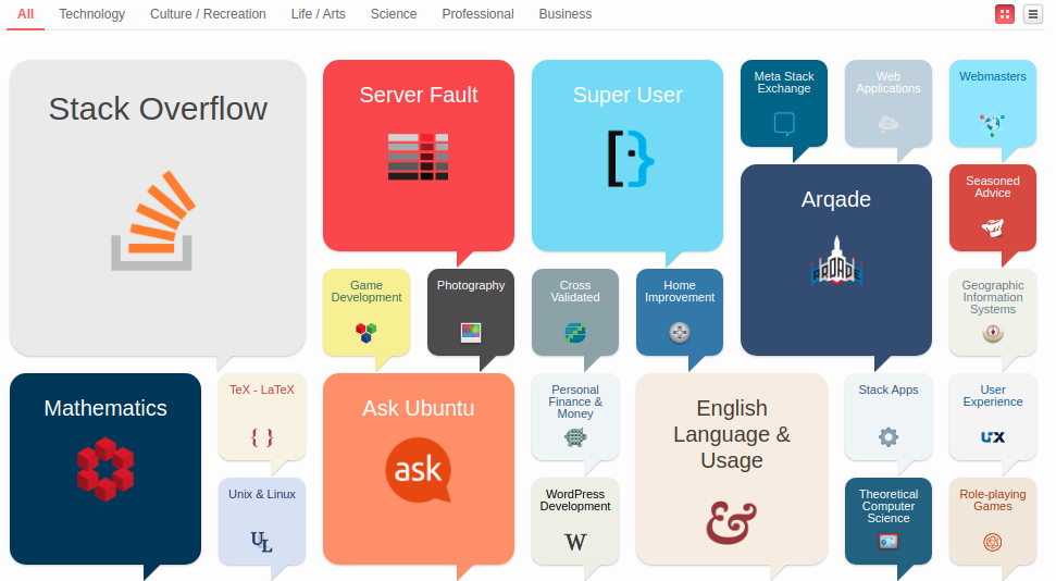
So how can we identify what topics in data science people are keen to learn about? The popular question and answer website network Stack Exchange may be of use here. Stack Exchange comprises a multitude of Q&A websites on topics across a diverse set of fields, with each site covering a specific topic. Some of the most popular sites are shown in the image below.
Lucky for us, there is one for data science:

The Data Science Stack Exchange (DSSE) site describes itself as:
a question and answer site for Data science professionals, Machine Learning specialists, and those interested in learning more about the field
Perfect. We also know from the Stack Exchange tour that anybody is able to ask a question, anybody can answer a question, and the best answers are voted up and rise to the top.
We should therefore be able to analyse the kinds of questions people are asking and see if there are any patterns in the topics being asked that could indicate areas of data science where the might be a knowledge gap, or a general lack of accessible educational material.
How is the DSSE website organised?

Here are the primary site sections:
Home- the homepage of the site, shown in the screenshot aboveQuestions- similar to the homepage, a list of all questions asked on the site, with numerous sorting options (newest, unanswered etc.)Tags- list of all tags used to categorise content on the site (these are the small, light-blue shaded boxes with labels)Users- list of all users active on the site, with links to their personal profilesUnanswered- list of all questions that currently have zero answers
We can see that questions on the DSSE usually have at least one tag (a category describing a specific area of data science). These tags look like they could be provide us with a means of analysing what questions are being asked, and will save us from having to categorise the questions ourselves.
Now that we have an idea of how we're going to analyse the data, the next step is to find a way of obtaining it!
Getting the data
Stack Exchange provides a public data base for each of its websites. We can explore and query the Data Science Stack Exchange's database using the Stack Exchange Data Explorer (SEDE).
At present, there are a total of 29 tables in the database. Here are a few which could be promising towards finding the most popular content:
Posts: contains data on every single non-deleted post, including both questions and answer postsTags: data on every tag that can be applied to a postComments: data on every comment left on a post - both question posts and answer posts can receive comments
Let's take a look at the Posts table in-depth. There are many columns in the Posts table, here are some that will likely be relevant to our goal:
Id: An identification number for the post.PostTypeId: An identification number for the type of post (explored in next section).CreationDate: The date and time of creation of the post.Score: The post's score (the sum of upvotes minus downvotes).ViewCount: How many times the post was viewed.Tags: What tags were applied to the post.AnswerCount: How many answers the question got (only applicable to question posts).FavoriteCount: How many times the question was favored (only applicable to question posts).
The Score, ViewCount, AnswerCount and FavouriteCount columns all contain data on how popular the post is—the kind of information we're after.
Post types
Let's investigate what types of post can be created. We can use the PostTypes table to see what post types are available and the IDs they correspond to.

There are eight different types of posts. Let's query the database with the following SQL to see how many of each type there are.
SELECT PostTypeId, COUNT(*) as NrOfPosts
  FROM posts
 GROUP BY PostTypeId;
| PostTypeId | NrOfPosts |
|---|---|
| 1 | 21446 |
| 2 | 23673 |
| 4 | 236 |
| 5 | 236 |
| 6 | 11 |
| 7 | 1 |
Question (PostTypeId 1) and Answer (PostTypeId 2) type questions make up the vast majority of all posts in the DSSE. Other post types are in relatively low volume. In any case, our analysis is based around trying to identify what people want to know about data science, and therefore, only the Question post type is relevant to us.
Recency is also important, we want any content we produce as a result of this analysis to be timely, and relevant to the questions on data science that people are asking now, rather than several years ago. We'll limit our analysis to posts created in the last full calendar year, which is 2021 (it's currently January 2022 at time of writing).
We'll query the Data Science Stack Exchange's database again using the following query to get our data:
SELECT Id,
       PostTypeId,
       CreationDate,
       Score,
       ViewCount,
       Tags,
       AnswerCount,
       FavoriteCount
  FROM Posts
 WHERE PostTypeId = 1 AND CreationDate LIKE '%2021%'
We'll import the CSV into a pandas dataframe and from there we can start exploring the data!
Importing the DSSE data and initial exploration
# import libraries
import pandas as pd
import numpy as np
import matplotlib.pyplot as plt
import seaborn as sns
# read in data from csv to pandas dataframe
questions = pd.read_csv("data_science_2021.csv", parse_dates=["CreationDate"])
# get a concise summary of the dataframe
questions.info()
<class 'pandas.core.frame.DataFrame'>
RangeIndex: 6581 entries, 0 to 6580
Data columns (total 8 columns):
 #   Column         Non-Null Count  Dtype
---  ------         --------------  -----
 0   Id             6581 non-null   int64
 1   PostTypeId     6581 non-null   int64
 2   CreationDate   6581 non-null   datetime64[ns]
 3   Score          6581 non-null   int64
 4   ViewCount      6581 non-null   int64
 5   Tags           6581 non-null   object
 6   AnswerCount    6581 non-null   int64
 7   FavoriteCount  557 non-null    float64
dtypes: datetime64[ns](1), float64(1), int64(5), object(1)
memory usage: 411.4+ KB
# view first and last five rows of dataset
display(questions.head())
display(questions.tail())
| Id | PostTypeId | CreationDate | Score | ViewCount | Tags | AnswerCount | FavoriteCount | |
|---|---|---|---|---|---|---|---|---|
| 0 | 92224 | 1 | 2021-03-27 03:49:05 | 1 | 120 | <classification><class-imbalance><nlp><bert> | 1 | NaN |
| 1 | 92227 | 1 | 2021-03-27 06:45:23 | 0 | 20 | <machine-learning><methodology> | 1 | NaN |
| 2 | 92230 | 1 | 2021-03-27 11:25:19 | 0 | 31 | <python><time-series><pandas><arima> | 0 | NaN |
| 3 | 92231 | 1 | 2021-03-27 12:00:06 | 1 | 132 | <time-series><autoencoder><anomaly-detection><... | 2 | NaN |
| 4 | 92235 | 1 | 2021-03-27 14:37:26 | 0 | 228 | <python><tensorflow><nlp><sentiment-analysis><... | 1 | NaN |
| Id | PostTypeId | CreationDate | Score | ViewCount | Tags | AnswerCount | FavoriteCount | |
|---|---|---|---|---|---|---|---|---|
| 6576 | 106589 | 1 | 2021-12-31 14:19:06 | 0 | 14 | <machine-learning><python><scikit-learn><data>... | 1 | NaN |
| 6577 | 106592 | 1 | 2021-12-31 15:49:20 | 1 | 35 | <deep-learning><overfitting> | 2 | NaN |
| 6578 | 106593 | 1 | 2021-12-31 19:41:13 | 1 | 58 | <feature-selection><markov-hidden-model> | 2 | NaN |
| 6579 | 106596 | 1 | 2021-12-31 22:37:42 | 1 | 18 | <machine-learning><linear-regression><cost-fun... | 1 | NaN |
| 6580 | 106598 | 1 | 2021-12-31 23:09:09 | 0 | 24 | <machine-learning><neural-network><predictive-... | 0 | NaN |
# count null values in each column
questions.isnull().sum()
Id                  0
PostTypeId          0
CreationDate        0
Score               0
ViewCount           0
Tags                0
AnswerCount         0
FavoriteCount    6024
dtype: int64
We can see that we have 6581 rows (i.e. 6581 individual questions) across 8 columns in our dataframe.
Only one column contains missing values, FavoriteCount - the number of times a post has been favored by a unique user. Infact, over 90% of the values in the FavoriteCount column are missing! It's probably safe to say that a missing value in this column is the equivalent of no users favoring the question, so we can replace the missing values with 0.
The FavoriteCount column is also the only column for which the datatype does not seem appropriate. Currently the data is stored as a Float. Given that the number of times a question is favored can only be a whole number, it would be best to store the data as an Int.
# replace missing values in FavoriteCount column with zero and convert column dtype to int
questions["FavoriteCount"] = questions["FavoriteCount"].fillna(0).astype(int)

# check dtypes of columns
questions.dtypes
Id                        int64
PostTypeId                int64
CreationDate     datetime64[ns]
Score                     int64
ViewCount                 int64
Tags                     object
AnswerCount               int64
FavoriteCount             int32
dtype: object
The only other column that might need amending is the Tags column. We know that the column values are stored as string, with each individual tag following the format <tag>. Each question on Stack Exchange can have up to a maximum of five tags, so we could potentially split out each tag into it's own column (Tag1 to Tag5), however, this would not help in relating tags between the individual questions. It's probably best that we keep all the data in one column, but modify the values slightly to a format that's easier to work with.
Clean Tags column
# clean the tags column into a list of comma-separated values
questions["Tags"] = (questions["Tags"].str.replace(r'^<|>$', "", regex=True) # strip first and last angle brackets
                                      .str.split("><") # split string on '><' to separate all the tags in the list
                    )

# check changes
questions["Tags"]
0            [classification, class-imbalance, nlp, bert]
1                         [machine-learning, methodology]
2                    [python, time-series, pandas, arima]
3       [time-series, autoencoder, anomaly-detection, ...
4       [python, tensorflow, nlp, sentiment-analysis, ...
                              ...
6576    [machine-learning, python, scikit-learn, data,...
6577                         [deep-learning, overfitting]
6578             [feature-selection, markov-hidden-model]
6579    [machine-learning, linear-regression, cost-fun...
6580    [machine-learning, neural-network, predictive-...
Name: Tags, Length: 6581, dtype: object
Now that the data has been cleaned, we can move on with analysis.
Analysis
One way we can determine what people want to know about in data science is by identifying the most popular tags. We'll use the following two proxies as a measure of 'popularity':
- the number of times the tag was used
- how many times a question with the tag was viewed
Let's start by determining the number of times each tag was used in a question post.
## determine the number times each tag was used ##

# get tags column and use explode() method to transform each element of a list into a new row
tag_used = questions["Tags"].explode("Tags")

# identify the count of each tag
tag_used = tag_used.value_counts()

# reset the index to get tags names as a column and rename the columns
tag_used = tag_used.reset_index().rename(columns={"index":"Tags", "Tags":"Used"})

# get a slice of the top 10 tags by times used
top_10_used = tag_used[:10]

top_10_used
| Tags | Used | |
|---|---|---|
| 0 | machine-learning | 1752 |
| 1 | python | 1207 |
| 2 | deep-learning | 950 |
| 3 | neural-network | 607 |
| 4 | nlp | 547 |
| 5 | classification | 531 |
| 6 | keras | 527 |
| 7 | tensorflow | 518 |
| 8 | time-series | 403 |
| 9 | scikit-learn | 370 |
Now let's plot this data on a bar chart.
## generate horizontal bar plot ##

fig, ax = plt.subplots(figsize=(10,10))
top_10_used.sort_values("Used").plot.barh(x="Tags",
                                              y="Used",
                                              legend=False,
                                              color="#2b826c",
                                              ax=ax)

# set title text and remove ylabel
plt.suptitle("Most questions on data science involve machine-learning",
             y=0.98, fontsize=19)
plt.title("Top 10 most frequently used tags by questions asked on the Data Science Stack Exchange in 2021",
          y=1.06, fontsize=13)
ax.set_ylabel(None)

# manually set tick labels
ax.set_xticks([0, 500, 1000, 1500, 2000])

# move xaxis ticks to top (makes them easier to see at a glance)
ax.xaxis.tick_top()

# add a vertical line down the centre tick label
ax.axvline(x=1000, ymin=0.02, c='grey', alpha=0.5)

# despine plot
for location in ['left', 'right', 'top', 'bottom']:
    ax.spines[location].set_visible(False)

# remove ticks marks
ax.tick_params(top=False, left=False)

# set xlabel tick colour to grey
ax.tick_params(axis='x', colors='grey')

# adjust the size of the tick labels
ax.tick_params(axis='both', labelsize=14)

plt.show()

Machine Learning, Python, and Deep Learning were the top 3 most-used tags on question posts in 2021. Now we can apply the same method to determine the number of times each tag was viewed.
## determine the number times each tag was viewed ##

tag_viewed = questions[["Tags", "ViewCount"]]
tag_viewed = tag_viewed.explode("Tags")
tag_viewed = (tag_viewed.groupby("Tags")["ViewCount"].sum()
                                                    .sort_values(ascending=False)
                                                    .reset_index()
             )

# get a slice of the top 10 tags by viewcount
top_10_viewed = tag_viewed[:10]

top_10_viewed
| Tags | ViewCount | |
|---|---|---|
| 0 | python | 161502 |
| 1 | machine-learning | 120442 |
| 2 | deep-learning | 80163 |
| 3 | keras | 67960 |
| 4 | tensorflow | 67927 |
| 5 | pandas | 53102 |
| 6 | scikit-learn | 52076 |
| 7 | nlp | 43963 |
| 8 | neural-network | 38556 |
| 9 | numpy | 35979 |
## generate horizontal bar plot ##

fig, ax = plt.subplots(figsize=(10,10))
top_10_viewed.sort_values("ViewCount").plot.barh(x="Tags",
                                              y="ViewCount",
                                              legend=False,
                                              color="#2b826c",
                                              ax=ax)

# set title text and remove ylabel
plt.suptitle("Questions tagged with Python were viewed more times than any other tag",
             y=0.98, fontsize=19)
plt.title("Top 10 tags by viewcount of questions asked on the Data Science Stack Exchange in 2021",
          y=1.06, fontsize=13)
ax.set_ylabel(None)

# manually set tick labels
ax.set_xticks([0, 80000, 160000])
ax.set_xticklabels(['0', '80,000', '160,000'])

# move xaxis ticks to top (makes them easier to see at a glance)
ax.xaxis.tick_top()

# add a vertical line down the centre tick label
ax.axvline(x=80000, ymin=0.02, c='grey', alpha=0.5)

# despine plot
for location in ['left', 'right', 'top', 'bottom']:
    ax.spines[location].set_visible(False)

# remove ticks marks
ax.tick_params(top=False, left=False)

# set xlabel tick colour to grey
ax.tick_params(axis='x', colors='grey')

# adjust the size of the tick labels
ax.tick_params(axis='both', labelsize=14)

Somewhat unsurprisingly, the top 3 most-viewed tags are the same as the top 3 most-used tags, though Python and Machine Learning have switched places.
Relationship between tags
We know from our exploration of the DSSE site earlier that multiple tags can be (and often are) used in a single post. It could be interesting to see whether some tags are frequently used together, and therefore are probably related to one-another in some way. As an example, looking at the graph of most-viewed tags, we know that pandas and numpy are both Python libraries and so will likely be used with the python tag.
To assess how many times a tag is used with another tag, we'll start by constructing an empty dataframe whereby each unique tag is listed along both the index and column axis.
# get list of each unique tag
unique_tags = list(tag_used["Tags"])

# create data frame using each tag as an index and a column
relation = pd.DataFrame(index=unique_tags, columns=unique_tags)

# fill dataframe with zeros
relation = relation.fillna(0)

# show sample of dataframe
relation.iloc[0:5, 0:5]
| machine-learning | python | deep-learning | neural-network | nlp | |
|---|---|---|---|---|---|
| machine-learning | 0 | 0 | 0 | 0 | 0 |
| python | 0 | 0 | 0 | 0 | 0 |
| deep-learning | 0 | 0 | 0 | 0 | 0 |
| neural-network | 0 | 0 | 0 | 0 | 0 |
| nlp | 0 | 0 | 0 | 0 | 0 |
Now that we have our dataframe (note that the dataframe above is just a small section of the entire dataframe!), we'll iterate over each list of tags in questions["Tags"], and using each list to index our dataframe, increment all the values in the returned slice of the dataframe by one. As an example for the first row:
first_list = ['classification', 'class-imbalance', 'nlp', 'bert']
relation.loc[first_list, first_list]
| classification | class-imbalance | nlp | bert | |
|---|---|---|---|---|
| classification | 0 | 0 | 0 | 0 |
| class-imbalance | 0 | 0 | 0 | 0 |
| nlp | 0 | 0 | 0 | 0 |
| bert | 0 | 0 | 0 | 0 |
We can then increment each value here by one as each tag was used with each other once. Now let's populate the relation dataframe.
# iterate over each list of tags
for tags in questions["Tags"]:
    # use the list of tags to lookup both the index and column and increment the value by one
    relation.loc[tags, tags] += 1

# display resulting dataframe
display(relation)
| machine-learning | python | deep-learning | neural-network | nlp | classification | keras | tensorflow | time-series | scikit-learn | ... | bernoulli | field-aware-factorization-machines | competitions | hashing | self-driving | lsi | spyder | bahdanau | mongodb | stata | |
|---|---|---|---|---|---|---|---|---|---|---|---|---|---|---|---|---|---|---|---|---|---|
| machine-learning | 1752 | 289 | 341 | 188 | 129 | 212 | 85 | 89 | 77 | 112 | ... | 0 | 0 | 0 | 0 | 0 | 0 | 0 | 0 | 0 | 0 |
| python | 289 | 1207 | 122 | 66 | 105 | 69 | 139 | 129 | 88 | 154 | ... | 0 | 0 | 0 | 0 | 0 | 0 | 1 | 0 | 0 | 0 |
| deep-learning | 341 | 122 | 950 | 190 | 75 | 60 | 147 | 144 | 48 | 11 | ... | 0 | 1 | 0 | 0 | 0 | 0 | 0 | 0 | 0 | 0 |
| neural-network | 188 | 66 | 190 | 607 | 26 | 38 | 85 | 62 | 28 | 11 | ... | 0 | 0 | 0 | 0 | 0 | 0 | 0 | 0 | 0 | 0 |
| nlp | 129 | 105 | 75 | 26 | 547 | 34 | 19 | 24 | 1 | 17 | ... | 0 | 0 | 0 | 0 | 0 | 0 | 0 | 0 | 0 | 0 |
| ... | ... | ... | ... | ... | ... | ... | ... | ... | ... | ... | ... | ... | ... | ... | ... | ... | ... | ... | ... | ... | ... |
| lsi | 0 | 0 | 0 | 0 | 0 | 0 | 0 | 0 | 0 | 0 | ... | 0 | 0 | 0 | 0 | 0 | 1 | 0 | 0 | 0 | 0 |
| spyder | 0 | 1 | 0 | 0 | 0 | 0 | 0 | 0 | 0 | 0 | ... | 0 | 0 | 0 | 0 | 0 | 0 | 1 | 0 | 0 | 0 |
| bahdanau | 0 | 0 | 0 | 0 | 0 | 0 | 0 | 0 | 1 | 0 | ... | 0 | 0 | 0 | 0 | 0 | 0 | 0 | 1 | 0 | 0 |
| mongodb | 0 | 0 | 0 | 0 | 0 | 0 | 0 | 0 | 0 | 0 | ... | 0 | 0 | 0 | 0 | 0 | 0 | 0 | 0 | 1 | 0 |
| stata | 0 | 0 | 0 | 0 | 0 | 0 | 0 | 0 | 0 | 0 | ... | 0 | 0 | 0 | 0 | 0 | 0 | 0 | 0 | 0 | 1 |
598 rows × 598 columns
Using this data we can see that, for example, python was used with machine-learning on 578 instances, and deep-learning was used with nlp 150 times. We can also see how many times an individual tag was used overall, for example python was used 1207 times.
This dataframe is too difficult to detect any patterns, so let's visualise this data in a heatmap. Before we do this, we should remove the values where a tag is "paired" with itself as this will skew the colours in the heatmap.
# remove values for when a tag matches itself
for value in relation.index:
    relation.loc[value, value] = np.NaN
The dataframe is also very large, so let's just focus on the top 10 most used tags for now
# create a slice of the relation dataframe with top 10 used tags
top_10 = relation.loc[top_10_used["Tags"], top_10_used["Tags"]]
Now let's create our heatmap
## plot heatmap
fig, ax = plt.subplots(figsize=(12,12))
ax = sns.heatmap(top_10, cmap="Greens")
plt.show()

It might be helpful to remove the upper triangle of this visual for clarity - we don't really need to see the same information twice. We'll also include the actual values for each tag-pairing.
# create a numpy array of zeros matching the dimensions of the top_10 df
mask = np.zeros_like(top_10)
# use triu_indicies to create the indices for the upper-triangle of an the array.
mask[np.triu_indices_from(mask)] = True

## plot heatmap
fig, ax = plt.subplots(figsize=(12,12))
ax = sns.heatmap(top_10,
                 cmap="Greens",
                 mask=mask,
                 annot=True,
                 fmt='g',
                 linewidths=.5,
                 annot_kws={"fontsize":14}) # we can now apply the mask

# set font-size for tick labels and rotate x tick labels
ax.tick_params(axis='both', which='major', labelsize=14)
ax.set_xticklabels(top_10.index, rotation = 45, ha="right")

# title
ax.set_title("Frequency of tag pairings", fontsize=16)

plt.show()

The heatmap provides us with some insight into how tags could be related. We can see that questions with the tag machine-learning are often paired with python and deep-learning. There also appears to be a connection between tensorflow and keras. It's important, however, to recognise that although these tags are often used with each other there isn't necessarily a relationship between the these pairings (i.e. using one tag may not increase [or decrease] the chance of using another tag). It could just be that because they are popular tags, they end up being used together.
The shortcomings of this method of analysing relationships between tags means we will have to rely on something else, domain knowledge!
Using domain knowledge
We'll do our own research to get a better understanding behind the tags, and use this knowledge to infer any relationships between tags. We can't reasonably do this for every tag, so instead we'll get a list of tags that appear in both the top 10 used and top 10 viewed lists we created earlier.
# inner join both top 10 used and top 10 viewed tag list to get only tags that appear in both
most_popular_tags = pd.merge(left=top_10_used, right=top_10_viewed, how="inner", left_on="Tags", right_on="Tags")
most_popular_tags
| Tags | Used | ViewCount | |
|---|---|---|---|
| 0 | machine-learning | 1752 | 120442 |
| 1 | python | 1207 | 161502 |
| 2 | deep-learning | 950 | 80163 |
| 3 | neural-network | 607 | 38556 |
| 4 | nlp | 547 | 43963 |
| 5 | keras | 527 | 67960 |
| 6 | tensorflow | 518 | 67927 |
| 7 | scikit-learn | 370 | 52076 |
So what exactly are these tags? Here's a brief description of each one based on our research:
machine-learninga branch of computer science and artificial intelligence involving the study of algorithms and data that can be used to 'train' a computer to make predictions or decisions without having to be explicitly programmed to do so, with accuracy improving as the computer continues to 'learn' from the data.python- a programming language commonly used in data science applications.deep-learninga subfield of machine learning, deep learning models exercise a greater deal of autonomy over classical machine learning methods, and learn in a way that is more similar to how a human would. Deep learning models are considered to be more scalable than classical machine learning, but require vast amounts of structured training data and processing power to achieve an acceptable level of accuracy.neural-network- a layered structure of algorithms that loosely mimic the network of neurons in the human brain, designed to recognise patterns in data. Neural networks form the basis of the majority of deep learning modelskeras- Keras is an open-source deep learning API developed by Google and written in Python, with the aim of making implementation of neural networks easy.classification- in the context of machine learning, classification is the process of predicting the class (i.e. category or label) of a given 'unclassified' data point. For example, an email spam detection model will attempt to classify an incoming email (the unknown data point) as either 'spam' or 'not spam', based on the training data it has been provided.nlp- natural language processing (NLP) is the branch of computer science and artificial intelligence concerned with enabling computers to understand human language, whether written or vocal. Common NLP tasks include speech recognition (interpreting voice data) and sentiment analysis (the detection of human emotion in language).tensorflow- TensorFlow is an open-source software library for machine learning and artificial intelligence. Like Keras, Tensorflow is a framework that aims to simplify the programming tasks involved in machine learningscikit-learn- a machine learning library for Python containing tools for predictive data analysis.
There is clearly a strong relationship between all these tags. With the exception of Python, they are all directly related to machine learning. More specifically, it's clear that the majority of tags are related to deep learning.
Let's take a deep dive on deep learning-related posts to see how suitable it is as a potential topic for our content.
Is deep learning just a fad?
Obviously we want the educational content we'll produce to have as much longevity as possible, so it's worth investigating whether interest in deep learning is increasing year on year, or if it's in decline.
We'll use the following query on the SEDE to get every question that has ever been asked on the DSSE. We'll limit it to the last full year, which was 2021.
SELECT Id, CreationDate, Tags
  FROM posts
 WHERE PostTypeId = 1 AND CreationDate < Convert(datetime, '2022');
This query will return the post ID, creation date, and tags, of all questions asked on DSSE before the year 2022.
Using this data, we can track the interest in deep learning across time. We will:
- Count how many deep learning questions are asked per time period.
- The total amount of questions per time period.
- How many deep learning questions there are relative to the total amount of questions per time period.
# import the csv generated by our SQL query
all_questions = pd.read_csv("all_questions.csv", parse_dates=["CreationDate"])

# identify minimum and maximum dates
print("Earliest date: ", all_questions["CreationDate"].min())
print("Last date: ", all_questions["CreationDate"].max())
Earliest date:  2014-05-13 23:58:30
Last date:  2021-12-31 23:09:09
We've got data ranging from mid-2014 to the end of 2021, this should give us a good insight into the evolution of deep-learning questions.
Clean tags column again
We'll need to clean the Tags column in our all_questions dataset as we did earlier with our questions dataset.
# clean the tags column into a list of comma-separated values
all_questions["Tags"] = (all_questions["Tags"].str.replace(r'^<|>$', "", regex=True) # strip first and last angle brackets
                                              .str.split("><") # split on '><' to get convert values into a list
                        )

# check changes
all_questions["Tags"]
0        [logistic-regression, data-science-model, opti...
1        [machine-learning, python, neural-network, ker...
2        [python, tensorflow, pytorch, normalization, b...
3         [clustering, statistics, descriptive-statistics]
4              [machine-learning, classification, xgboost]
                               ...
31529                           [machine-learning, python]
31530                                                [cnn]
31531                               [python, scikit-learn]
31532    [machine-learning, multiclass-classification, ...
31533                                    [r, missing-data]
Name: Tags, Length: 31534, dtype: object
Now we can begin analysing these tags, but first, we need to identify what actually counts as a 'deep learning question'.
Defining what a 'deep learning' question is
In order to get any further with our analysis, we will need to come up with a definition for what counts as a 'deep learning question'.
The easiest solution would be to use use the most popular tags we identified earlier on, taking the ones that are specifically related to deep learning. An obvious caveat to this approach is that there could potentially be more deep learning-related tags that were not among the most popular tags we identified earlier; however, we know that the most popular tags will have the greatest impact on our analysis.
Here are the tags we've identified as having a strong connection to deep-learning:
deep-learning- no surprise!neural-network- neural networks are a core part of deep learningkeras- assists with the implementation of neural networkstensorflow- although tensorflow can be used for a variety of machine learning tasks, it has a particular focus on deep neural networks
# list of tags directly related to deep learning
deep_tags = ["deep-learning",
             "neural-network",
             "keras",
             "tensorflow",
            ]

# function to identify rows containing tags related to deep learning
def deep_learning(tag_list, dl_tags):
    if any(x in tag_list for x in dl_tags): # any() returns True if any item in an iterable equals True
        return 1
    else:
        return 0

# apply function to 'Tags' column and asign result to new column called deep_learning
all_questions["deep_learning"] = all_questions["Tags"].apply(deep_learning, dl_tags=deep_tags)

all_questions["deep_learning"].value_counts()
0    22660
1     8874
Name: deep_learning, dtype: int64
We can see that across all time, there are 8874 deep learning questions and 22,660 non-deep learning questions, so nearly 30% of all questions asked on the DSSE are related to deep learning!
While that sounds promising, we need to know how the share of questions related to deep-learning has evolved over time. First, we need a suitable time period to analyse our data over. At the moment, we have the exact creation date of each question. This would too granular for our needs, so we'll create a new column containing the quarter and year a question was created (e.g. 2021Q1). It might also be nice to group the data by year alone, so we'll do that too.
# use PeriodIndex function to get date by quarter and year
all_questions["quarter"] = pd.PeriodIndex(all_questions["CreationDate"], freq='Q')

# extract just the year alone
all_questions["year"] = all_questions["CreationDate"].dt.to_period('Y')

all_questions
| Id | CreationDate | Tags | deep_learning | quarter | year | |
|---|---|---|---|---|---|---|
| 0 | 89817 | 2021-02-23 16:52:48 | [logistic-regression, data-science-model, opti... | 0 | 2021Q1 | 2021 |
| 1 | 89818 | 2021-02-23 18:09:14 | [machine-learning, python, neural-network, ker... | 1 | 2021Q1 | 2021 |
| 2 | 89819 | 2021-02-23 18:39:55 | [python, tensorflow, pytorch, normalization, b... | 1 | 2021Q1 | 2021 |
| 3 | 89820 | 2021-02-23 19:01:34 | [clustering, statistics, descriptive-statistics] | 0 | 2021Q1 | 2021 |
| 4 | 89823 | 2021-02-23 20:26:11 | [machine-learning, classification, xgboost] | 0 | 2021Q1 | 2021 |
| ... | ... | ... | ... | ... | ... | ... |
| 31529 | 41788 | 2018-11-28 12:07:18 | [machine-learning, python] | 0 | 2018Q4 | 2018 |
| 31530 | 41795 | 2018-11-28 13:47:59 | [cnn] | 0 | 2018Q4 | 2018 |
| 31531 | 41797 | 2018-11-28 14:31:42 | [python, scikit-learn] | 0 | 2018Q4 | 2018 |
| 31532 | 41798 | 2018-11-28 14:35:57 | [machine-learning, multiclass-classification, ... | 0 | 2018Q4 | 2018 |
| 31533 | 41799 | 2018-11-28 16:04:28 | [r, missing-data] | 0 | 2018Q4 | 2018 |
31534 rows × 6 columns
Now that we have the dates we need, let's aggregate the deep_learning column by the quarter and by year columns.
# create pivot table counting instances of deep learning and non-deep learning questions by month-year
all_pv = all_questions.pivot_table(values="Id", columns='deep_learning', index=["year", "quarter"], aggfunc='count')

## reshape pivot table into a typical dataframe for easier use ##

# remove unwanted axis name
remove_label = all_pv.rename_axis(None, axis=1)

# reset index and rename columns to something more intuitive
dl_questions = remove_label.reset_index().rename(columns={0:"non-dl_q", 1:"dl_q"})

dl_questions
| year | quarter | non-dl_q | dl_q | |
|---|---|---|---|---|
| 0 | 2014 | 2014Q2 | 150 | 7 |
| 1 | 2014 | 2014Q3 | 180 | 8 |
| 2 | 2014 | 2014Q4 | 199 | 15 |
| 3 | 2015 | 2015Q1 | 175 | 13 |
| 4 | 2015 | 2015Q2 | 264 | 20 |
| 5 | 2015 | 2015Q3 | 282 | 28 |
| 6 | 2015 | 2015Q4 | 327 | 52 |
| 7 | 2016 | 2016Q1 | 431 | 79 |
| 8 | 2016 | 2016Q2 | 432 | 78 |
| 9 | 2016 | 2016Q3 | 456 | 119 |
| 10 | 2016 | 2016Q4 | 379 | 139 |
| 11 | 2017 | 2017Q1 | 483 | 207 |
| 12 | 2017 | 2017Q2 | 447 | 186 |
| 13 | 2017 | 2017Q3 | 504 | 203 |
| 14 | 2017 | 2017Q4 | 611 | 277 |
| 15 | 2018 | 2018Q1 | 769 | 430 |
| 16 | 2018 | 2018Q2 | 958 | 458 |
| 17 | 2018 | 2018Q3 | 892 | 554 |
| 18 | 2018 | 2018Q4 | 863 | 403 |
| 19 | 2019 | 2019Q1 | 1223 | 510 |
| 20 | 2019 | 2019Q2 | 1264 | 522 |
| 21 | 2019 | 2019Q3 | 1249 | 493 |
| 22 | 2019 | 2019Q4 | 1037 | 462 |
| 23 | 2020 | 2020Q1 | 1287 | 489 |
| 24 | 2020 | 2020Q2 | 1233 | 494 |
| 25 | 2020 | 2020Q3 | 1024 | 420 |
| 26 | 2020 | 2020Q4 | 851 | 357 |
| 27 | 2021 | 2021Q1 | 1107 | 462 |
| 28 | 2021 | 2021Q2 | 1328 | 574 |
| 29 | 2021 | 2021Q3 | 1153 | 441 |
| 30 | 2021 | 2021Q4 | 1102 | 374 |
Now we need to determine the percentage of questions that are related to deep-learning for each time period.
dl_questions["total_q"] = dl_questions["non-dl_q"] + dl_questions["dl_q"]

dl_questions["dl_pct"] = round(dl_questions["dl_q"] / dl_questions["total_q"] * 100, 2)

pd.set_option('display.max_rows', 10)
dl_questions.sort_values("dl_pct", ascending=False)
| year | quarter | non-dl_q | dl_q | total_q | dl_pct | |
|---|---|---|---|---|---|---|
| 17 | 2018 | 2018Q3 | 892 | 554 | 1446 | 38.31 |
| 15 | 2018 | 2018Q1 | 769 | 430 | 1199 | 35.86 |
| 16 | 2018 | 2018Q2 | 958 | 458 | 1416 | 32.34 |
| 18 | 2018 | 2018Q4 | 863 | 403 | 1266 | 31.83 |
| 14 | 2017 | 2017Q4 | 611 | 277 | 888 | 31.19 |
| ... | ... | ... | ... | ... | ... | ... |
| 4 | 2015 | 2015Q2 | 264 | 20 | 284 | 7.04 |
| 2 | 2014 | 2014Q4 | 199 | 15 | 214 | 7.01 |
| 3 | 2015 | 2015Q1 | 175 | 13 | 188 | 6.91 |
| 0 | 2014 | 2014Q2 | 150 | 7 | 157 | 4.46 |
| 1 | 2014 | 2014Q3 | 180 | 8 | 188 | 4.26 |
31 rows × 6 columns
Let's start with a simple graph of the percentage share of deep learning questions to get a rough idea of the interest in deep learning over time. To do this we'll need to get the average dl_pct for each year.
# get mean dl_pct for each year
year_avg_dl_pct = dl_questions.groupby("year")["dl_pct"].mean()

# plot graph
fig, ax = plt.subplots(figsize=(15,10))
year_avg_dl_pct.plot(x="year",
                     y="dl_pct",
                     c="orange",
                     marker="o",
                     ax=ax)

ax.set_title("Percentage share of deep learning questions asked on DSSE over time",
             fontsize=20)

# remove spines
for location in ['left', 'right', 'bottom', 'top']:
    ax.spines[location].set_visible(False)

# remove ticks
ax.tick_params(left=False, bottom=False)

# adjust tick label size
ax.tick_params(axis='both', which='major', labelsize=13)

# set y labels, hide x label
ax.set_ylabel('Pct', size=14)
ax.set_xlabel('')

plt.show()

We can see that deep learning peaked in 2018, and has since started to trail off a bit. Let's explore this data in more detail by looking at both the percentage share and volume of deep learning questions asked at a quarterly level.
fig, ax = plt.subplots(figsize=(15,10))

# generate bar plot
ax1 = dl_questions.plot.bar(x="quarter",
                            y="dl_q",
                            ax=ax,
                            width=0.5,
                            label='volume', # set label for legend
                            color="#2b826c"
                           )

# generate line plot
ax2 = dl_questions.plot(x="quarter",
                  y="dl_pct",
                  linewidth=2.5,
                  c="orange",
                  ax=ax,
                  rot=90,
                  secondary_y=True,
                  use_index=False, # necessary to force line plot on same axes as bar plot
                                  # when index of df is datetime/period (as bar plots are categorical, not continous)
                  label='percent',
                  marker="o"
                 )

# remove spines
for location in ['left', 'right', 'bottom', 'top']:
    ax1.spines[location].set_visible(False)
    ax2.spines[location].set_visible(False)

# remove ticks
ax.tick_params(left=False, bottom=False)
ax2.tick_params(right=False)

# adjust tick label size
ax.tick_params(axis='both', which='major', labelsize=13)
ax.tick_params(axis='both', which='minor', labelsize=10)
ax2.tick_params(axis='y', labelsize=13)

# hide x ticks
ax.set_xticks([])

# remove x-axis label
ax.set_xlabel(None)

# set y labels
ax1.set_ylabel('Volume', size=14)
ax2.set_ylabel('Pct share', size=14)

ax.set_title("Volume and percentage share of deep learning questions asked on DSSE by quarter",
             fontsize=20,
            x=0.5, y=1.1)

## create vertical guides that indicate year

xpos = [2,6,10,14,18,22,26]
years = dl_questions["year"].unique()

for i, year in zip(xpos, years[1:]): # slice 2014 off since it's not a full year
    ax.axvline(x=i+0.75, alpha=0.2)
    ax.text(x=i+0.9, y=570, rotation="vertical", s=year, size=12)

## manually create legend handles for easier control

import matplotlib.patches as mpatches

# create legend handles
blue_patch = mpatches.Patch(color='#2b826c', label='Volume')
orange_patch = mpatches.Patch(color='orange', label='Percent share')

# plot legend
ax.legend(handles=[blue_patch, orange_patch], loc="upper center", bbox_to_anchor=(0.5, 1.09),
          ncol=2, fancybox=True, shadow=True)

plt.show()

We can see that the percentage share of deep learning related questions continuously increased year on year (with 2016 seeing the largest YoY growth) until a peak in 2018, where over 40% of all questions on the DSSE website where related to deep learning. Since 2018, the share of deep learning questions has dropped, though the volume of questions asked has remained fairly consistent.
Interestingly, if we use the Google Trends tool to analyse the popularity of the search term 'deep learning' on Google Search, using the same time window as the chart above, the pattern is very similar to what we see in our DSSE data. The peak popularity of 'deep learning' as a Google Search query also hit it's peak in 2018 too around a similar time, plateauing and then declining in 2021.

Conclusion
machine-learning,python, anddeep-learningwere observed to be both the most used and most viewed tags on the entire DSSE for the year 2021- the peak percentage share of deep-learning related questions was
38%in the third quarter of 2018, with an anual average of35%. - 2019 saw a large drop in percentage share, reducing to
29%and then remaining in a slight decline through to 2021 - although the percentage share of deep-learning related questions has been in decline since 2018, the actual volume of questions has remained fairly consistent since 2018
- overall, we would recommend commissioning content related deep learning - while interest may be in a slight decline, it is clearly still a very popular area of data science