CSC321H5 Project 3.
Deadline: Thursday, March. 19, by 9pm
Submission: Submit a PDF export of the completed notebook.
Late Submission: Please see the syllabus for the late submission criteria.
In this assignment, we will build a convolutional neural network that can predict whether two shoes are from the same pair or from two different pairs. This kind of application can have real-world applications: for example to help people who are visually impaired to have more independence.
We will explore two convolutional architectures. While we will give you starter code to help make data processing a bit easier, you'll have a chance to build your neural network all by yourself!
You may modify the starter code as you see fit, including changing the signatures of functions and adding/removing helper functions. However, please make sure that your TA can understand what you are doing and why.
If you find exporting the Google Colab notebook to be difficult, you can create your own PDF report that includes your code, written solutions, and outputs that the graders need to assess your work.
import pandas
import numpy as np
import matplotlib.pyplot as plt

import torch
import torch.nn as nn
import torch.optim as optim
Question 1. Data
Download the data from the course website at https://www.cs.toronto.edu/~lczhang/321/files/p3data.zip
Unzip the file. There are three
main folders: train, test_w and test_m. Data in train will be used for
training and validation, and the data in the other folders will be used for testing.
This is so that the entire class will have the same test sets.
We've separated test_w and test_m so that we can track our model performance
for women's shoes and men's shoes separately. Each of the test sets contain images
from 10 students who submitted images of either exclusively men's shoes or women's
shoes.
Upload this data to Google Colab. Then, mount Google Drive from your Google Colab notebook:
from google.colab import drive
drive.mount('/content/gdrive')
After you have done so, read this entire section (ideally this entire handout) before proceeding. There are right and wrong ways of processing this data. If you don't make the correct choices, you may find yourself needing to start over. Many machine learning projects fail because of the lack of care taken during the data processing stage.
Part (a) -- 1 pts
Why might we care about the accuracies of the men's and women's shoes as two separate measures? Why would we expect our model accuracies for the two groups to be different?
Recall that your application may help people who are visually impaired.
# Your answer goes here. Please make sure it is not cut off
Part (b) -- 4 pts
Load the training and test data, and separate your training data into training and validation.
Create the numpy arrays train_data, valid_data, test_w and test_m, all of which should
be of shape [*, 3, 2, 224, 224, 3]. The dimensions of these numpy arrays are as follows:
*- the number of students allocated to train, valid, or test3- the 3 pairs of shoes submitted by that student2- the left/right shoes224- the height of each image224- the width of each image3- the colour channels
So, the item train_data[4,0,0,:,:,:] should give us the left shoe of the first image submitted
by the 5th student.The item train_data[4,0,1,:,:,:] should be the right shoe in the same pair.
The item train_data[4,1,1,:,:,:] should be the right shoe in a different pair, submitted by
the same student.
When you first load the images using (for example) plt.imread, you may see a numpy array of shape
[224, 224, 4] instead of [224, 224, 3]. That last channel is the alpha channel for transparent
pixels, and should be removed.
The pixel intensities are stored as an integer between 0 and 255.
Divide the intensities by 255 so that you have floating-point values between 0 and 1. Then, subtract 0.5
so that the elements of train_data, valid_data and test_data are between -0.5 and 0.5.
Note that this step actually makes a huge difference in training!
This function might take a while to run---it takes 3-4 minutes for me to just load the files from Google Drive. If you want to avoid running this code multiple times, you can save your numpy arrays and load it later: https://docs.scipy.org/doc/numpy/reference/generated/numpy.save.html
# Your code goes here. Make sure it does not get cut off
# You can use the code below to help you get started. You're welcome to modify
# the code or remove it entirely: it's just here so that you don't get stuck
# reading files

import glob
path = "/content/gdrive/My Drive/CSC321/data/train/*.jpg" # edit me
images = {}
for file in glob.glob(path):
    filename = file.split("/")[-1]   # get the name of the .jpg file
    img = plt.imread(file)           # read the image as a numpy array
    images[filename] = img[:, :, :3] # remove the alpha channel
# Run this code, include the image in your PDF submission
# plt.figure()
# plt.imshow(train_data[4,0,0,:,:,:]) # left shoe of first pair submitted by 5th student
# plt.figure()
# plt.imshow(train_data[4,0,1,:,:,:]) # right shoe of first pair submitted by 5th student
# plt.figure()
# plt.imshow(train_data[4,1,1,:,:,:]) # right shoe of second pair submitted by 5th student
Part (c) -- 2 pts
Since we want to train a model that determines whether two shoes come from the same pair or different pairs, we need to create some labelled training data. Our model will take in an image, either consisting of two shoes from the same pair or from different pairs. So, we'll need to generate some positive examples with images containing two shoes that are from the same pair, and some negative examples where images containing two shoes that are not from the same pair. We'll generate the positive examples in this part, and the negative examples in part (c).
Write a function generate_same_pair() that takes one of the data sets that you produced
in part (a), and generates a numpy array where each pair of shoes in the data set is
concatenated together. In particular, we'll be concatenating together images of left
and right shoes along the height axis. Your function generate_same_pair should
return a numpy array of shape [*, 448, 224, 3].
(Later on, we will need to convert this numpy array into a PyTorch tensor with shape
[*, 3, 448, 224]. For now, we'll keep the RGB channel as the last dimension since
that's what plt.imshow requires)
# Your code goes here

# Run this code, include the result with your PDF submission
print(train_data.shape) # if this is [N, 3, 2, 224, 224, 3]
print(generate_same_pair(train_data).shape) # should be [N*3, 448, 224, 3]
plt.imshow(generate_same_pair(train_data)[0]) # should show 2 shoes from the same pair
Part (d) -- 2 pts
Write a function generate_different_pair() that takes one of the data sets that
you produced in part (a), and generates a numpy array in the same shape as part (b).
However, each image will contain 2 shoes from a different pair, but submitted
by the same student. Do this by jumbling the 3 pairs of shoes submitted by
each student.
Theoretically, for each student image submissions, there are 6 different combinations
of "wrong pairs" that we could produce. To keep our data set balanced, we will
only produce three combinations of wrong pairs per unique person.
In other words,generate_same_pairs and generate_different_pairs should
return the same number of training examples.
# Your code goes here

# Run this code, include the result with your PDF submission
print(train_data.shape) # if this is [N, 3, 2, 224, 224, 3]
print(generate_different_pair(train_data).shape) # should be [N*3, 448, 224, 3]
plt.imshow(generate_different_pair(train_data)[0]) # should show 2 shoes from different pairs
Part (e) -- 1 pts
Why do we insist that the different pairs of shoes still come from the same student? (Hint: what else do images from the same student have in common?)
# Your answer goes here. Please make sure it is not cut off
Part (f) -- 1 pts
Why is it important that our data set be balanced? In other words suppose we created a data set where 99% of the images are of shoes that are not from the same pair, and 1% of the images are shoes that are from the same pair. Why could this be a problem?
# Your answer goes here. Please make sure it is not cut off
Question 2. Convolutional Neural Networks
Before starting this question, we recommend reviewing the lecture and tutorial materials on convolutional neural networks.
In this section, we will build two CNN models in PyTorch.
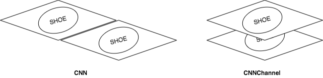
Part (a) -- 4 pts
Implement a CNN model in PyTorch called CNN that will take images of size
$3 \times 448 \times 224$, and classify whether the images contain shoes from
the same pair or from different pairs.
The model should contain the following layers:
- A convolution layer that takes in 3 channels, and outputs $n$ channels.
- A $2 \times 2$ downsampling (either using a strided convolution in the previous step, or max pooling)
- A second convolution layer that takes in $n$ channels, and outputs $n \times 2$ channels.
- A $2 \times 2$ downsampling (either using a strided convolution in the previous step, or max pooling)
- A third convolution layer that takes in $n \times 2$ channels, and outputs $n \times 4$ channels.
- A $2 \times 2$ downsampling (either using a strided convolution in the previous step, or max pooling)
- A fourth convolution layer that takes in $n \times 4$ channels, and outputs $n \times 8$ channels.
- A $2 \times 2$ downsampling (either using a strided convolution in the previous step, or max pooling)
- A fully-connected layer with 100 hidden units
- A fully-connected layer with 2 hidden units
Make the variable $n$ a parameter of your CNN. You can use either $3 \times 3$ or $5 \times 5$
convolutions kernels. Set your padding to be (kernel_size - 1) / 2 so that your feature maps
have an even height/width.
Note that we are omitting certain steps that practitioners will typically not mention, like ReLU activations and reshaping operations. Use the tutorial materials and your past projects to figure out where they are.
class CNN(nn.Module):
    def __init__(self, n=4):
        super(CNN, self).__init__()
        # TODO: complete this method

    # TODO: complete this class
Part (b) -- 4 pts
Implement a CNN model in PyTorch called CNNChannel that contains the same layers as
in the Part (a), but with one crucial difference: instead of starting with an image
of shape $3 \times 448 \times 224$, we will first manipulate the image so that the
left and right shoes images are concatenated along the channel dimension.
Complete the manipulation in the forward() method (by slicing and using
the function torch.cat). The input to the first convolutional layer
should have 6 channels instead of 3 (input shape $6 \times 224 \times 224$).
Use the same hyperparameter choices as you did in part (a), e.g. for the kernel size, choice of downsampling, and other choices.
class CNNChannel(nn.Module):
    def __init__(self, n=4):
        super(CNNChannel, self).__init__()
        # TODO: complete this method

    # TODO: complete this class
Part (c) -- 2 pts
Although our task is a binary classification problem, we will still use the architecture
of a multi-class classification problem. That is, we'll use a one-hot vector to represent
our target (just like in Project 2). We'll also use CrossEntropyLoss instead of
BCEWithLogitsLoss. In fact, this is a standard practice in machine learning because
this architecture performs better!
Explain why this architecture might give you better performance.
# Your answer goes here. Please make sure it is not cut off
Part (d) -- 2 pts
The two models are quite similar, and should have almost the same number of parameters. However, one of these models will perform better, showing that architecture choices do matter in machine learning. Explain why one of these models performs better.
# Your answer goes here. Please make sure it is not cut off
Part (e) -- 2 pts
The function get_accuracy is written for you. You may need to modify this
function depending on how you set up your model and training.
Unlike in project 2, we will separately compute the model accuracy on the positive and negative samples. Explain why we may wish to track these two values separately.
# Your answer goes here. Please make sure it is not cut off
def get_accuracy(model, data, batch_size=50):
    """Compute the model accuracy on the data set. This function returns two
    separate values: the model accuracy on the positive samples,
    and the model accuracy on the negative samples.

    Example Usage:

    >>> model = CNN() # create untrained model
    >>> pos_acc, neg_acc= get_accuracy(model, valid_data)
    >>> false_positive = 1 - pos_acc
    >>> false_negative = 1 - neg_acc
    """

    model.eval()
    n = data.shape[0]

    data_pos = generate_same_pair(data)      # should have shape [n * 3, 448, 224, 3]
    data_neg = generate_different_pair(data) # should have shape [n * 3, 448, 224, 3]

    pos_correct = 0
    for i in range(0, len(data_pos), batch_size):
        xs = torch.Tensor(data_pos[i:i+batch_size]).transpose(1, 3)
        zs = model(xs)
        pred = zs.max(1, keepdim=True)[1] # get the index of the max logit
        pred = pred.detach().numpy()
        pos_correct += (pred == 1).sum()

    neg_correct = 0
    for i in range(0, len(data_neg), batch_size):
        xs = torch.Tensor(data_neg[i:i+batch_size]).transpose(1, 3)
        zs = model(xs)
        pred = zs.max(1, keepdim=True)[1] # get the index of the max logit
        pred = pred.detach().numpy()
        neg_correct += (pred == 0).sum()

    return pos_correct / (n * 3), neg_correct / (n * 3)
Question 3. Training
Now, we will write the functions required to train the model.
Part (a) -- 10 pts
Write the function train_model that takes in (as parameters) the model, training data,
validation data, and other hyperparameters like the batch size, weight decay, etc.
This function should be somewhat similar to the training code that you wrote
in Project 2, but with a major difference in the way we treat our training data.
Since our positive and negative training sets are separate, it is actually easier for
us to generate separate minibatches of positive and negative training data! In
each iteration, we'll take batch_size / 2 positive samples and batch_size / 2
negative samples. We will also generate labels of 1's for the positive samples,
and 0's for the negative samples.
Here's what we will be looking for:
- main training loop; choice of loss function; choice of optimizer
- obtaining the positive and negative samples
- shuffling the positive and negative samples at the start of each epoch
- in each iteration, take
batch_size / 2positive samples andbatch_size / 2negative samples as our input for this batch - in each iteration, take
np.ones(batch_size / 2)as the labels for the positive samples, andnp.zeros(batch_size / 2)as the labels for the negative samples - conversion from numpy arrays to PyTorch tensors, making sure that the input has dimensions "NCHW",
use the
.transpose()method in either PyTorch or numpy - computing the forward and backward passes
- after every epoch, checkpoint your model (Project 2 has in-depth instructions and examples for how to do this)
- after every epoch, report the accuracies for the training set and validation set
- track the training curve information and plot the training curve
# Write your code here
Part (b) -- 2 pts
Sanity check your code from Q3(a) and from Q2(a) and Q2(b) by showing that your models can memorize a very small subset of the training set (e.g. 5 images). You should be able to achieve 90%+ accuracy relatively quickly (within ~30 or so iterations).
(If you have trouble with CNN() but not CNNChannel(), try reducing $n$, e.g. try working
with the model CNN(2))
# Write your code here. Remember to include your results so that your TA can
# see that your model attains a high training accuracy. (UPDATED March 12)
Part (c) -- 4 pts
Train your models from Q2(a) and Q2(b). You will want to explore the effects of a few hyperparameters, including the learning rate, batch size, choice of $n$, and potentially the kernel size. You do not need to check all values for all hyperparameters. Instead, get an intuition about what each of the parameters do.
In this section, explain how you tuned your hyperparameters.
# Include the training curves for the two models.
Part (d) -- 2 pts
Include your training curves for the best models from each of Q2(a) and Q2(b). These are the models that you will use in Question 4.
# Include the training curves for the two models.
Question 4.
Part (a) -- 3 pts
Report the test accuracies of your single best model, separately for the two test sets. Do this by choosing the checkpoint of the model architecture that produces the best validation accuracy. That is, if your model attained the best validation accuracy in epoch 12, then the weights at epoch 12 is what you should be using to report the test accuracy.
# Write your code here. Make sure to include the test accuracy in your report
Part (b) -- 2 pts
Display one set of men's shoes that your model correctly classified as being from the same pair.
If your test accuracy was not 100% on the men's shoes test set, display one set of inputs that your model classified incorrectly.
Part (c) -- 2 pts
Display one set of women's shoes that your model correctly classified as being from the same pair.
If your test accuracy was not 100% on the women's shoes test set, display one set of inputs that your model classified incorrectly.