ENV/ATM 415: Climate Laboratory
Brian E. J. Rose, University at Albany
Lecture 16: The one-dimensional Energy Balance Model
Way back at the beginning of the semester we wrote down a global average energy budget that looked like
$$ C \frac{dT}{dt} = \text{ASR} - \text{OLR} $$Last time we talked about the additional local heating of each latitude band associated with atmospheric and oceanic motions:
$$ h = - \frac{1}{2 \pi a^2 \cos\phi } \frac{\partial \mathcal{H}}{\partial \phi} $$Using this, we can write down a local energy budget expressing how the temperature of each latitude band should change:
$$ C \frac{\partial T}{\partial t} = \text{ASR} - \text{OLR} - \frac{1}{2 \pi a^2 \cos\phi } \frac{\partial \mathcal{H}}{\partial \phi}$$Now the temperature $T$ is a function of latitude $\phi$ as well as time $t$ (so we write it as a partial derivative)
We also introduced the diffusive heat transport parameterization
$$ \mathcal{H}(\phi) = -2 \pi ~a^2 \cos\phi D \frac{\partial T}{\partial \phi} $$Putting this parameterization into the budget above gives
$$ C \frac{\partial T}{\partial t} = \text{ASR} - \text{OLR} + \frac{D}{\cos\phi } \frac{\partial}{\partial \phi} \left( \cos\phi \frac{\partial T}{\partial \phi} \right)$$(where we pulled the parameter $D$ out of the derivative because we are assuming it is a constant)
To turn our budget into a model, we need specific parameterizations that link the radiation ASR and OLR to surface temperature $T$ (the state variable for our model).
Fixed albedo assumption
First, as usual, we can write the solar term as
$$ \text{ASR} = (1-\alpha) ~ Q $$For now, we will assume that the planetary albedo is fixed (does not depend on temperature). Therefore the entire shortwave term $(1-\alpha) Q$ is a fixed source term in our budget. It varies in space and time but does not depend on $T$.
Note that the solar term is (at least in annual average) larger at equator than poles… and transport term acts to flatten out the temperatures.
Parameterizing the longwave radiation
Now, we almost have a model we can solve for $T$! Just need a function OLR$(T)$ expressing the temperature dependence of the emission to space.
So… what’s the link between OLR and temperature????
[ discuss ]
We spent a good chunk of the course looking at this question, and developed a model of a vertical column of air.
We are trying now to build a model of the equator-to-pole (or pole-to-pole) temperature structure.
We COULD use an array of column models, representing temperature as a function of height and latitude (and time).
But instead, we will keep things simple, one spatial dimension at a time.
Introduce the following simple parameterization:
$$ \text{OLR} = A + B T $$With:
- $T$ the zonal average surface temperature in ºC
- $A$ is a constant in W m$^{-2}$
- $B$ is a constant in W m$^{-2}$ ºC$^{-1}$.
Think of $A$ as an inverse measure of the greenhouse gas amount (Why?).
The parameter $B$ is closely related to the climate feedback parameter $\lambda$ that we defined a while back. The only difference is that in the EBM we are going to explicitly separate the albedo feedback from all other radiative feedbacks.
OLR versus surface temperature in NCEP Reanalysis data
Let's look at the data to find reasonable values for $A$ and $B$.
%matplotlib inline
import numpy as np
import matplotlib.pyplot as plt
import xarray as xr
import climlab
ncep_url = "http://www.esrl.noaa.gov/psd/thredds/dodsC/Datasets/ncep.reanalysis.derived/"
ncep_air = xr.open_dataset( ncep_url + "pressure/air.mon.1981-2010.ltm.nc", decode_times=False)
ncep_Ts = xr.open_dataset( ncep_url + "surface_gauss/skt.sfc.mon.1981-2010.ltm.nc", decode_times=False)
lat_ncep = ncep_Ts.lat; lon_ncep = ncep_Ts.lon
print( ncep_Ts)
<xarray.Dataset>
Dimensions:             (lat: 94, lon: 192, nbnds: 2, time: 12)
Coordinates:
  * lon                 (lon) float32 0.0 1.875 3.75 5.625 7.5 9.375 11.25 ...
  * time                (time) float64 -6.571e+05 -6.57e+05 -6.57e+05 ...
  * lat                 (lat) float32 88.542 86.6531 84.7532 82.8508 80.9473 ...
Dimensions without coordinates: nbnds
Data variables:
    climatology_bounds  (time, nbnds) float64 ...
    skt                 (time, lat, lon) float64 ...
    valid_yr_count      (time, lat, lon) float64 ...
Attributes:
    title:                          4x daily NMC reanalysis
    description:                    Data is from NMC initialized reanalysis\n...
    platform:                       Model
    Conventions:                    COARDS
    not_missing_threshold_percent:  minimum 3% values input to have non-missi...
    history:                        Created 2011/07/12 by doMonthLTM\nConvert...
    References:                     http://www.esrl.noaa.gov/psd/data/gridded...
    dataset_title:                  NCEP-NCAR Reanalysis 1
Ts_ncep_annual = ncep_Ts.skt.mean(dim=('lon','time'))
ncep_ulwrf = xr.open_dataset( ncep_url + "other_gauss/ulwrf.ntat.mon.1981-2010.ltm.nc", decode_times=False)
ncep_dswrf = xr.open_dataset( ncep_url + "other_gauss/dswrf.ntat.mon.1981-2010.ltm.nc", decode_times=False)
ncep_uswrf = xr.open_dataset( ncep_url + "other_gauss/uswrf.ntat.mon.1981-2010.ltm.nc", decode_times=False)
OLR_ncep_annual = ncep_ulwrf.ulwrf.mean(dim=('lon','time'))
ASR_ncep_annual = (ncep_dswrf.dswrf - ncep_uswrf.uswrf).mean(dim=('lon','time'))
from scipy.stats import linregress
slope, intercept, r_value, p_value, std_err = linregress(Ts_ncep_annual, OLR_ncep_annual)

print( 'Best fit is A = %0.0f W/m2 and B = %0.1f W/m2/degC' %(intercept, slope))
Best fit is A = 214 W/m2 and B = 1.6 W/m2/degC
We're going to plot the data and the best fit line, but also another line using these values:
#  More standard values
A = 210.
B = 2.
fig, ax1 = plt.subplots(figsize=(8,6))
ax1.plot( Ts_ncep_annual, OLR_ncep_annual, 'o' , label='data')
ax1.plot( Ts_ncep_annual, intercept + slope * Ts_ncep_annual, 'k--', label='best fit')
ax1.plot( Ts_ncep_annual, A + B * Ts_ncep_annual, 'r--', label='B=2')
ax1.set_xlabel('Surface temperature (C)', fontsize=16)
ax1.set_ylabel('OLR (W m$^{-2}$)', fontsize=16)
ax1.set_title('OLR versus surface temperature from NCEP reanalysis', fontsize=18)
ax1.legend(loc='upper left')
ax1.grid()

Discuss these curves...
Suggestion of at least 3 different regimes with different slopes (cold, medium, warm).
Unbiased "best fit" is actually a poor fit over all the intermediate temperatures.
The astute reader will note that... by taking the zonal average of the data before the regression, we are biasing this estimate toward cold temperatures. [WHY?]
Let's take these reference values:
$$ A = 210 ~ \text{W m}^{-2}, ~~~ B = 2 ~ \text{W m}^{-2}~^\circ\text{C}^{-1} $$Note that in the global average, recall $\overline{T_s} = 288 \text{ K} = 15^\circ\text{C}$
And so this parameterization gives
$$ \overline{\text{OLR}} = 210 + 15 \times 2 = 240 ~\text{W m}^{-2} $$And the observed global mean is $\overline{\text{OLR}} = 239 ~\text{W m}^{-2} $ So this is consistent.
Relationship between $B$ and feedback parameters
Recall that when we looked at climate forcing and feedback, we said that overall response to a forcing $\Delta R$ in W m$^{-2}$ is
$$ \Delta T = \frac{\Delta R}{\lambda} $$and where $\lambda$ is the overall climate feedback parameter:
$$\lambda = \lambda_0 - \sum_{i=1}^{N} \lambda_i $$and
- $\lambda_0 = 3.3$ W m$^{-2}$ K$^{-1}$ is the no-feedback climate response
- $\sum_{i=1}^{N} \lambda_i$ is the sum of all radiative feedbacks, defined to be positive for amplifying processes.
More positive feedbacks thus mean that $\lambda$ is a smaller number, which means the response to a given forcing is larger!
Here in the EBM the parameter $B$ plays the same role as $\lambda$ -- a smaller number means a more sensitive model.
Our estimate $B = 2 ~ \text{W m}^{-2}~^\circ\text{C}^{-1}$ thus implies that the sum of all LW feedback processes (including water vapor, lapse rates and clouds) is
$$ \sum_{i=1}^{N} \lambda_i = 3.3 ~\text{W m}^{-2}~^\circ\text{C}^{-1} - 2 ~\text{W m}^{-2}~^\circ\text{C}^{-1} = 1.3 ~\text{W m}^{-2}~^\circ\text{C}^{-1} $$Looking back at the chart of feedback parameter values from GCMs, does this seem plausible?
Putting the above OLR parameterization into our budget equation gives
$$ C \frac{\partial T}{\partial t} = (1-\alpha) ~ Q - \left( A + B~T \right) + \frac{D}{\cos\phi } \frac{\partial }{\partial \phi} \left( \cos\phi ~ \frac{\partial T}{\partial \phi} \right) $$This is the equation for a very important and useful simple model of the climate system. It is typically referred to as the (one-dimensional) Energy Balance Model.
(although as we have seen over and over, EVERY climate model is actually an “energy balance model” of some kind)
Also for historical reasons this is often called the Budyko-Sellers model, after Budyko and Sellers who both (independently of each other) published influential papers on this subject in 1969.
Recap: parameters in this model are
- C: heat capacity in J m$^{-2}$ ºC$^{-1}$
- A: longwave emission at 0ºC in W m$^{-2}$
- B: increase in emission per degree, in W m$^{-2}$ ºC$^{-1}$
- D: horizontal (north-south) diffusivity of the climate system in W m$^{-2}$ ºC$^{-1}$
We also need to specify the albedo.
Tune albedo formula to match observations
Let's go back to the NCEP Reanalysis data to see how planetary albedo actually varies as a function of latitude.
days = np.linspace(1.,50.)/50 * climlab.constants.days_per_year
Qann_ncep = np.mean( climlab.solar.insolation.daily_insolation(lat_ncep, days ),axis=1)
albedo_ncep = 1 - ASR_ncep_annual / Qann_ncep

albedo_ncep_global = np.average(albedo_ncep, weights=np.cos(np.deg2rad(lat_ncep)))
print( 'The annual, global mean planetary albedo is %0.3f' %albedo_ncep_global)
fig,ax = plt.subplots()
ax.plot(lat_ncep, albedo_ncep)
ax.grid();
ax.set_xlabel('Latitude')
ax.set_ylabel('Albedo')
The annual, global mean planetary albedo is 0.354
Text(0,0.5,'Albedo')

The albedo increases markedly toward the poles.
There are several reasons for this:
- surface snow and ice increase toward the poles
- Cloudiness is an important (but complicated) factor.
- Albedo increases with solar zenith angle (the angle at which the direct solar beam strikes a surface)
Approximating the observed albedo
The albedo curve can be approximated by a smooth function that increases with latitude:
$$ \alpha(\phi) \approx \alpha_0 + \alpha_2 P_2(\sin\phi) $$where $P_2$ is a function called the 2nd Legendre polynomial. Don't worry about exactly what this means. This is what it looks like:
# Add a new curve to the previous figure
a0 = albedo_ncep_global
a2 = 0.25
ax.plot(lat_ncep, a0 + a2 * climlab.utils.legendre.P2(np.sin(np.deg2rad(lat_ncep))))
fig

Of course we are not fitting all the details of the observed albedo curve. But we do get the correct global mean a reasonable representation of the equator-to-pole gradient in albedo.
For now, we will be focusing on the annual mean model.
For the insolation, we set $Q(\phi,t) = \bar{Q}(\phi)$, the annual mean value (large at equator, small at pole).
Animating the adjustment of annual mean EBM to equilibrium
Before looking at the details of how to set up an EBM in climlab, let's look at an animation of the adjustment of the model (its temperature and energy budget) from an isothermal initial condition.
For reference, all the code necessary to generate the animation is here in the notebook.
#  Some imports needed to make and display animations
from IPython.display import HTML
from matplotlib import animation

def setup_figure():
    templimits = -20,32
    radlimits = -340, 340
    htlimits = -6,6
    latlimits = -90,90
    lat_ticks = np.arange(-90,90,30)

    fig, axes = plt.subplots(3,1,figsize=(8,10))
    axes[0].set_ylabel('Temperature (deg C)')
    axes[0].set_ylim(templimits)
    axes[1].set_ylabel('Energy budget (W m$^{-2}$)')
    axes[1].set_ylim(radlimits)
    axes[2].set_ylabel('Heat transport (PW)')
    axes[2].set_ylim(htlimits)
    axes[2].set_xlabel('Latitude')
    for ax in axes: ax.set_xlim(latlimits); ax.set_xticks(lat_ticks); ax.grid()
    fig.suptitle('Diffusive energy balance model with annual-mean insolation', fontsize=14)
    return fig, axes

def initial_figure(model):
    #  Make figure and axes
    fig, axes = setup_figure()
    # plot initial data
    lines = []
    lines.append(axes[0].plot(model.lat, model.Ts)[0])
    lines.append(axes[1].plot(model.lat, model.ASR, 'k--', label='SW')[0])
    lines.append(axes[1].plot(model.lat, -model.OLR, 'r--', label='LW')[0])
    lines.append(axes[1].plot(model.lat, model.net_radiation, 'c-', label='net rad')[0])
    lines.append(axes[1].plot(model.lat, model.heat_transport_convergence(), 'g--', label='dyn')[0])
    lines.append(axes[1].plot(model.lat,
        np.squeeze(model.net_radiation)+model.heat_transport_convergence(), 'b-', label='total')[0])
    axes[1].legend(loc='upper right')
    lines.append(axes[2].plot(model.lat_bounds, model.diffusive_heat_transport())[0])
    lines.append(axes[0].text(60, 25, 'Day 0'))
    return fig, axes, lines

def animate(day, model, lines):
    model.step_forward()
    #  The rest of this is just updating the plot
    lines[0].set_ydata(model.Ts)
    lines[1].set_ydata(model.ASR)
    lines[2].set_ydata(-model.OLR)
    lines[3].set_ydata(model.net_radiation)
    lines[4].set_ydata(model.heat_transport_convergence())
    lines[5].set_ydata(np.squeeze(model.net_radiation)+model.heat_transport_convergence())
    lines[6].set_ydata(model.diffusive_heat_transport())
    lines[-1].set_text('Day {}'.format(int(model.time['days_elapsed'])))
    return lines
#  A model starting from isothermal initial conditions
e = climlab.EBM_annual()
e.Ts[:] = 15.  # in degrees Celsius
e.compute_diagnostics()
#  Plot initial data
fig, axes, lines = initial_figure(e)

ani = animation.FuncAnimation(fig, animate, frames=np.arange(1, 100), fargs=(e, lines))
HTML(ani.to_html5_video())
We want to choose a value of $D$ that gives a reasonable approximation to observations:
- $\Delta T \approx 45$ ºC between equator and pole
- $\mathcal{H}_{max} \approx 5.5$ PW (peak heat transport)
ebm = climlab.EBM_annual(num_lat=40, A=210, B=2, a0=0.354, a2=0.25, D=1.)
print(ebm)
climlab Process of type <class 'climlab.model.ebm.EBM_annual'>.
State variables and domain shapes:
  Ts: (40, 1)
The subprocess tree:
Untitled: <class 'climlab.model.ebm.EBM_annual'>
   LW: <class 'climlab.radiation.aplusbt.AplusBT'>
   insolation: <class 'climlab.radiation.insolation.AnnualMeanInsolation'>
   albedo: <class 'climlab.surface.albedo.P2Albedo'>
   diffusion: <class 'climlab.dynamics.diffusion.MeridionalDiffusion'>
ebm.integrate_years(20.)
Integrating for 1800 steps, 7304.844000000001 days, or 20.0 years.
Total elapsed time is 19.99999999999943 years.
ebm.Ts
Field([[-12.26380533],
       [-11.90335191],
       [-11.18600118],
       [-10.11933409],
       [ -8.71602774],
       [ -6.99587506],
       [ -4.99120883],
       [ -2.7496105 ],
       [ -0.32575346],
       [  2.22075802],
       [  4.82660239],
       [  7.4259771 ],
       [  9.95205275],
       [ 12.33865448],
       [ 14.52211192],
       [ 16.44318978],
       [ 18.04899789],
       [ 19.29477742],
       [ 20.14546523],
       [ 20.57694989],
       [ 20.57694989],
       [ 20.14546524],
       [ 19.29477743],
       [ 18.04899791],
       [ 16.44318981],
       [ 14.52211196],
       [ 12.33865452],
       [  9.9520528 ],
       [  7.42597714],
       [  4.82660244],
       [  2.22075807],
       [ -0.3257534 ],
       [ -2.74961044],
       [ -4.99120876],
       [ -6.995875  ],
       [ -8.71602768],
       [-10.11933402],
       [-11.18600112],
       [-11.90335184],
       [-12.26380526]])
deltaT = np.max(ebm.Ts) - np.min(ebm.Ts)
print(deltaT)
32.84075522594018
#. The heat transport in PW
ebm.heat_transport()
array([ -0.00000000e+00,  -9.18904284e-02,  -3.64621108e-01,
        -8.09080950e-01,  -1.40900546e+00,  -2.13887046e+00,
        -2.95710444e+00,  -3.80557880e+00,  -4.62917406e+00,
        -5.37363147e+00,  -5.98702816e+00,  -6.42232424e+00,
        -6.64021012e+00,  -6.61185866e+00,  -6.32125688e+00,
        -5.76684312e+00,  -4.96224035e+00,  -3.93595867e+00,
        -2.73003339e+00,  -1.39766258e+00,  -1.04149739e-08,
         1.39766256e+00,   2.73003337e+00,   3.93595865e+00,
         4.96224033e+00,   5.76684310e+00,   6.32125687e+00,
         6.61185864e+00,   6.64021011e+00,   6.42232423e+00,
         5.98702816e+00,   5.37363146e+00,   4.62917406e+00,
         3.80557879e+00,   2.95710444e+00,   2.13887046e+00,
         1.40900546e+00,   8.09080950e-01,   3.64621108e-01,
         9.18904284e-02,  -0.00000000e+00])
# what's the peak value?
np.max(ebm.heat_transport())
6.6402101078967064
Class exercise
Repeat these calculations with some different values of $D$. We'll crowd-source the optimal value that best matches our observational targets.
Results
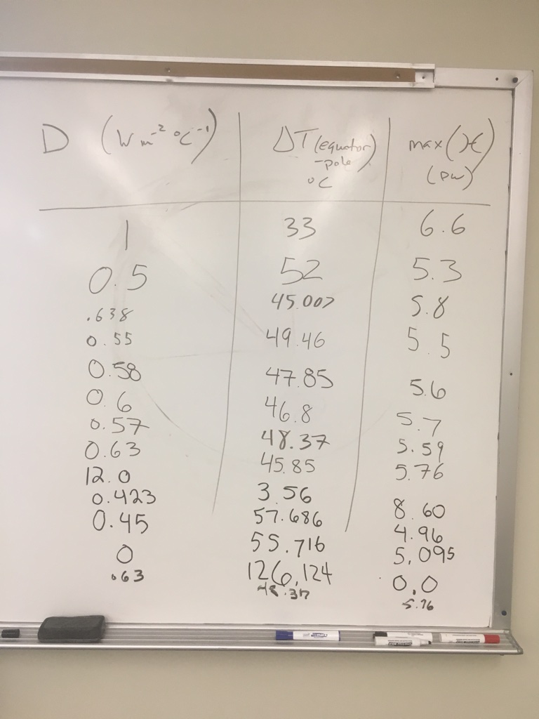
12 students calculated $\Delta T$ and $\mathcal{H}_{max}$ for different values of the diffusivity parameter $D$.
We collected the data on the whiteboard during class:
Here are the same data entered into a Pandas data frame.
import pandas as pd
classdata = pd.DataFrame({'$D$': [1., 0.5, 0.638, 0.55, 0.58, 0.6, 0.57, 0.63, 12.0, 0.423, 0.45, 0., 0.63],
                          '$\Delta T$': [33., 52., 45.007, 49.46, 47.85, 46.8, 48.37, 45.85, 3.56, 57.686, 55.716, 126.124, 48.37],
                          '$\mathcal{H}_{max}$': [6.6, 5.3, 5.8, 5.5, 5.6, 5.7, 5.59, 5.76, 8.60, 4.96, 5.095, 0., 5.76],
                         })
classdata
| $D$ | $\Delta T$ | $\mathcal{H}_{max}$ | |
|---|---|---|---|
| 0 | 1.000 | 33.000 | 6.600 |
| 1 | 0.500 | 52.000 | 5.300 |
| 2 | 0.638 | 45.007 | 5.800 |
| 3 | 0.550 | 49.460 | 5.500 |
| 4 | 0.580 | 47.850 | 5.600 |
| 5 | 0.600 | 46.800 | 5.700 |
| 6 | 0.570 | 48.370 | 5.590 |
| 7 | 0.630 | 45.850 | 5.760 |
| 8 | 12.000 | 3.560 | 8.600 |
| 9 | 0.423 | 57.686 | 4.960 |
| 10 | 0.450 | 55.716 | 5.095 |
| 11 | 0.000 | 126.124 | 0.000 |
| 12 | 0.630 | 48.370 | 5.760 |
Now we can do fun things like make a scatterplot of the data:
fig, axes = plt.subplots(2,1)
classdata.plot.scatter(x='$D$', y='$\Delta T$', ax=axes[0])
classdata.plot.scatter(x='$D$', y='$\mathcal{H}_{max}$', ax=axes[1])
<matplotlib.axes._subplots.AxesSubplot at 0x121666198>

Evidently the temperature gradient $\Delta T$ decreases with $D$, while the heat transport increases with $D$.
A more systematic search
Darray = np.arange(0., 2.05, 0.05)

model_list = []
Tmean_list = []
deltaT_list = []
Hmax_list = []

for D in Darray:
    ebm = climlab.EBM_annual(A=210, B=2, a0=0.354, a2=0.25, D=D)
    ebm.integrate_years(20., verbose=False)
    Tmean = ebm.global_mean_temperature()
    deltaT = np.max(ebm.Ts) - np.min(ebm.Ts)
    energy_in = np.squeeze(ebm.ASR - ebm.OLR)
    Htrans = ebm.heat_transport()
    Hmax = np.max(Htrans)
    model_list.append(ebm)
    Tmean_list.append(Tmean)
    deltaT_list.append(deltaT)
    Hmax_list.append(Hmax)
color1 = 'b'
color2 = 'r'

fig, ax1 = plt.subplots(figsize=(8,6))
ax1.plot(Darray, deltaT_list, color=color1)
ax1.plot(Darray, Tmean_list, 'b--')
ax1.set_xlabel('D (W m$^{-2}$ K$^{-1}$)', fontsize=14)
ax1.set_xticks(np.arange(Darray[0], Darray[-1], 0.2))
ax1.set_ylabel('$\Delta T$ (equator to pole)', fontsize=14,  color=color1)
for tl in ax1.get_yticklabels():
    tl.set_color(color1)
ax2 = ax1.twinx()
ax2.plot(Darray, Hmax_list, color=color2)
ax2.set_ylabel('Maximum poleward heat transport (PW)', fontsize=14, color=color2)
for tl in ax2.get_yticklabels():
    tl.set_color(color2)
ax1.set_title('Effect of diffusivity on temperature gradient and heat transport in the EBM', fontsize=16)
#  Add our crowd-sourced data to the figure
classdata.plot.scatter(x='$D$', y='$\Delta T$', ax=ax1)
classdata.plot.scatter(x='$D$', y='$\mathcal{H}_{max}$', ax=ax2)
for ax in [ax1, ax2]:
    ax.set_xlim(0,2)
ax1.plot([0.6, 0.6], [0, 140], 'k-')
ax1.grid()

When $D=0$, every latitude is in radiative equilibrium and the heat transport is zero. As we have already seen, this gives an equator-to-pole temperature gradient much too high.
When $D$ is large, the model is very efficient at moving heat poleward. The heat transport is large and the temperture gradient is weak.
The real climate seems to lie in a sweet spot in between these limits.
It looks like our fitting criteria are met reasonably well with $D=0.6$ W m$^{-2}$ K$^{-1}$
Also, note that the global mean temperature (plotted in dashed blue) is completely insensitive to $D$. Why do you think this is so?
Our model is defined by the following equation
$$ C \frac{\partial T}{\partial t} = (1-\alpha) ~ Q - \left( A + B~T \right) + \frac{D}{\cos\phi } \frac{\partial }{\partial \phi} \left( \cos\phi ~ \frac{\partial T}{\partial \phi} \right) $$with the albedo given by
$$ \alpha(\phi) = \alpha_0 + \alpha_2 P_2(\sin\phi) $$We have chosen the following parameter values, which seems to give a reasonable fit to the observed annual mean temperature and energy budget:
- $ A = 210 ~ \text{W m}^{-2}$
- $ B = 2 ~ \text{W m}^{-2}~^\circ\text{C}^{-1} $
- $ a_0 = 0.354$
- $ a_2 = 0.25$
- $ D = 0.6 ~ \text{W m}^{-2}~^\circ\text{C}^{-1} $