Table of Contents
- 1 Madonna di Canneto
- 2 Water spring Madonna di Canneto
- 2.1 Methodology
- 2.2 Rainfall
- 2.2.1 Soil moisture condition
- 2.2.2 TR-55: 'Urban Hydrology for Small Watersheds'
- 2.2.3 SCS CN- or curve number method
- 2.2.4 Runoff curve numbers for cultivated/other agricultural lands and soil types
- 2.2.5 Calculate runoff depth
- 2.2.6 The determination of CN values: by formula method, or by conversion table method
- 2.3 Temperature
- 2.4 Flow rate
- 2.5 Solar Radiation
- 2.6 Prediction of flow rate Madonna di Canneto source
Madonna di Canneto
Can you help preserve "blue gold" using data to predict water availability?
Acea Smart Water Analytics
https://www.kaggle.com/c/acea-water-prediction/data
Data Description
This competition uses nine different datasets, completely independent and not linked to each other. Each dataset can represent a different kind of waterbody. As each waterbody is different from the other, the related features as well are different from each other. So, if for instance we consider a water spring we notice that its features are different from the lake’s one. This is correct and reflects the behavior and characteristics of each waterbody. The Acea Group deals with four different type of waterbodies: water spring (for which three datasets are provided), lake (for which a dataset is provided), river (for which a dataset is provided) and aquifers (for which four datasets are provided).
Let’s see how these nine waterbodies differ from each other.
Aquifer
Auser
- This waterbody consists of two subsystems, called NORTH and SOUTH, where the former partly influences the behavior of the latter. Indeed, the north subsystem is a water table (or unconfined) aquifer while the south subsystem is an artesian (or confined) groundwater. The levels of the NORTH sector are represented by the values of the SAL, PAG, CoS and DIEC wells, while the levels of the SOUTH sector by the LT2 well.
Petrignano Aquifer
- The wells field of the alluvial plain between Ospedalicchio di Bastia Umbra and Petrignano is fed by three underground aquifers separated by low permeability septa. The aquifer can be considered a water table groundwater and is also fed by the Chiascio river. The groundwater levels are influenced by the following parameters: rainfall, depth to groundwater, temperatures and drainage volumes, level of the Chiascio river.
Doganella Aquifer
- The wells field Doganella is fed by two underground aquifers not fed by rivers or lakes but fed by meteoric infiltration. The upper aquifer is a water table with a thickness of about 30m. The lower aquifer is a semi-confined artesian aquifer with a thickness of 50m and is located inside lavas and tufa products. These aquifers are accessed through wells called Well 1, ..., Well 9. Approximately 80 % of the drainage volumes come from the artesian aquifer. The aquifer levels are influenced by the following parameters: rainfall, humidity, subsoil, temperatures and drainage volumes.
Luco Aquifer
- The Luco wells field is fed by an underground aquifer. This aquifer not fed by rivers or lakes but by meteoric infiltration at the extremes of the impermeable sedimentary layers. Such aquifer is accessed through wells called Well 1, Well 3 and Well 4 and is influenced by the following parameters: rainfall, depth to groundwater, temperature and drainage volumes.
Water spring
Amiata
- The Amiata waterbody is composed of a volcanic aquifer not fed by rivers or lakes but fed by meteoric infiltration. This aquifer is accessed through Ermicciolo, Arbure, Bugnano and Galleria Alta water springs. The levels and volumes of the four sources are influenced by the parameters: rainfall, depth to groundwater, hydrometry, temperatures and drainage volumes.
Madonna di Canneto
- The Madonna di Canneto spring is situated at an altitude of 1010m above sea level in the Canneto valley. It does not consist of an aquifer and its source is supplied by the water catchment area of the river Melfa.
- Settefrati is a commune with an altitude of 784 m and surface area of 50,6 km².
Lupa
- this water spring is located in the Rosciano Valley, on the left side of the Nera river. The waters emerge at an altitude of about 375 meters above sea level through a long draining tunnel that crosses, in its final section, lithotypes and essentially calcareous rocks. It provides drinking water to the city of Terni and the towns around it.
River
Arno
- Arno is the second largest river in peninsular Italy and the main waterway in Tuscany and it has a relatively torrential regime, due to the nature of the surrounding soils (marl and impermeable clays). Arno results to be the main source of water supply of the metropolitan area of Florence-Prato-Pistoia. The availability of water for this waterbody is evaluated by checking the hydrometric level of the river at the section of Nave di Rosano.
Lake
Bilancino
- Bilancino lake is an artificial lake located in the municipality of Barberino di Mugello (about 50 km from Florence). It is used to refill the Arno river during the summer months. Indeed, during the winter months, the lake is filled up and then, during the summer months, the water of the lake is poured into the Arno river.
Each waterbody has its own different features to be predicted. The table below shows the expected feature to forecast for each waterbody.
It is of the utmost importance to notice that some features like rainfall and temperature, which are present in each dataset, don’t go alongside the date. Indeed, both rainfall and temperature affect features like level, flow, depth to groundwater and hydrometry some time after it fell down. This means, for instance, that rain fell on 1st January doesn’t affect the mentioned features right the same day but some time later. As we don’t know how many days/weeks/months later rainfall affects these features, this is another aspect to keep into consideration when analyzing the dataset.
A short, tabular description of the waterbodies is available also downloading all datasets.
More information about the behavior of each kind of waterbody can be found at the following links:
- Aquifer https://en.wikipedia.org/wiki/Aquifer
- Water spring https://en.wikipedia.org/wiki/Spring_(hydrology)
- River https://en.wikipedia.org/wiki/River
- Lake https://en.wikipedia.org/wiki/Lake
import numpy as np
import matplotlib.pyplot as plt
import seaborn as sns
import pandas as pd
sns.set()
sns.set_context('notebook')
np.set_printoptions(threshold=20, precision=2, suppress=True)
pd.options.display.max_rows = 57
pd.options.display.max_columns = 38
pd.set_option('precision', 2)
from IPython.display import Image, display
%config InlineBackend.figure_format = 'retina';
from IPython.core.display import display, HTML, SVG
display(HTML("<style>.container {width:70% !important;}</style>"))
#sns.axes_style()
{'axes.facecolor': '#EAEAF2',
'axes.edgecolor': 'white',
'axes.grid': True,
'axes.axisbelow': True,
'axes.labelcolor': '.15',
'figure.facecolor': 'white',
'grid.color': 'white',
'grid.linestyle': '-',
'text.color': '.15',
'xtick.color': '.15',
'ytick.color': '.15',
'xtick.direction': 'out',
'ytick.direction': 'out',
'lines.solid_capstyle': <CapStyle.round: 'round'>,
'patch.edgecolor': 'w',
'patch.force_edgecolor': True,
'image.cmap': 'rocket',
'font.family': ['sans-serif'],
'font.sans-serif': ['Arial',
'DejaVu Sans',
'Liberation Sans',
'Bitstream Vera Sans',
'sans-serif'],
'xtick.bottom': False,
'xtick.top': False,
'ytick.left': False,
'ytick.right': False,
'axes.spines.left': True,
'axes.spines.bottom': True,
'axes.spines.right': True,
'axes.spines.top': True}
imgValle= Image( url="http://vanoproy.be/css/Valle_Canneto-Irto-Bellaveduta-RoccaAltiera.jpg", width=1300) # http://vanoproy.be/css filename
imgInfil= Image( url="http://vanoproy.be/python/figs/evaporation_infiltration_en.png", width=500)
imgValle

This map of VdC I found on a website reporting a daylong hike, which trail is imaged by the blue trace. The water spring itself surfaces on the right side of the valley, near the 1025 m notation.
South of the peak Monti della Meta there is a "plateau", a quasi horizontal surface with some local depressions, which can serve as a supplementory infiltration area for the water spring.
I can imaging there is some underground connection as dissolving calcium could have made conduits, while earthquakes and tectonics could have made cracks in the rocks.
Introduction: the study of springs
In recent years, long and frequent droughts have affected many countries in the world. These events require an ever more careful and rational management of water resources. Most of the globe’s unfrozen freshwater reserves are stored in aquifers. Groundwater is generally a renewable resource that shows good quality and resilience to fluctuations. Thus, if properly managed, groundwater could ensure long-term supply in order to meet increasing water demand.
For this purpose, it is of crucial importance to be able to predict the flow rates provided by springs. These represent the transitions from groundwater to surface water and reflect the dynamics of the aquifer, with the whole flow system behind. Moreover, spring influences water bodies into which they discharge. The importance of springs in groundwater research is highlighted in some significant contributions. In-depth studies on springs started only after the concept of sustainability was introduced in the management of water resources.
A spring hydrograph is the consequence of several processes governing the transformation of precipitation in the spring recharge area into the single output discharge at the spring. A water balance states that the change rate in water stored in the feeding aquifer is balanced by the rate at which water flows into and out of the aquifer. A quantitative water balance generally has to take the following terms into account: precipitation, infiltration, surface runoff, evapotranspiration, groundwater recharge, soil moisture deficit, spring discharge, lateral inflow to the aquifer, leakage between the aquifer and the underlying aquitard, well pumpage from the aquifer, and change of the storage in the aquifer.
In many cases, the evaluation of the terms of the water balance is very complicated. The complexity of the problem arises from many factors: hydrologic, hydrographic, and hydrogeological features, geologic and geomorphologic characteristics, land use, land cover, water withdrawals, and climatic conditions.
Even more complicated would be to estimate future spring discharges by using a model based on the balance equations. Therefore, simplified approaches are frequently pursued for practical purposes.
Many authors have addressed the problem of correlating the spring discharges to the rainfall through different approaches...
Note: you can skip the earthquake chapter, as these phenomenon are unpredictable. However, closeby earthquakes have an influence: they do distort the data.
Earthquakes =pd.read_csv(r"earthquake_15_20_EMSC.csv",header=0, sep=",", engine='python', encoding="UTF-8",parse_dates=True );
Earthquakes["Date"] = pd.to_datetime( Earthquakes.Date, format='%Y/%m/%d' , ) # euro dates utc=True
Earthquakes.set_index("Date", inplace=True)
Earthquakes["Dst"] = np.sqrt(np.abs((41.683364-Earthquakes.Latitude ) )+ np.abs((13.910494 -Earthquakes.Longitude)))#**2 **2
Earthquakes.nlargest(19, "Magnitude")
| Time UTC | Latitude | Longitude | Depth | Depth Type | Magnitude Type | Magnitude | Region Name | Last Update | Eqid | Dst | |
|---|---|---|---|---|---|---|---|---|---|---|---|
| Date | |||||||||||
| 2019-06-23 | 20:43:48 | 41.86 | 12.77 | 9 | f | ML | 3.7 | SOUTHERN ITALY | 2019-06-24 03:07 | 772989 | 1.15 |
| 2017-02-03 | 21:33:03 | 41.05 | 12.72 | 2 | ML | 3.7 | SOUTHERN ITALY | 2017-02-04 13:22 | 564948 | 1.35 | |
| 2017-02-03 | 23:08:05 | 41.01 | 12.69 | 2 | ML | 3.5 | SOUTHERN ITALY | 2017-02-04 13:21 | 564959 | 1.38 | |
| 2018-12-29 | 23:52:48 | 41.87 | 12.78 | 10 | f | ML | 2.9 | SOUTHERN ITALY | 2018-12-30 19:51 | 735792 | 1.15 |
| 2017-10-25 | 13:35:55 | 41.56 | 13.19 | 11 | f | ML | 2.9 | SOUTHERN ITALY | 2017-10-25 13:46 | 626212 | 0.92 |
| 2017-09-28 | 06:57:15 | 41.53 | 12.95 | 5 | ML | 2.8 | SOUTHERN ITALY | 2017-09-28 07:10 | 620966 | 1.06 | |
| 2017-02-04 | 02:10:42 | 41.07 | 12.68 | 11 | f | ML | 2.8 | SOUTHERN ITALY | 2017-02-04 02:29 | 565004 | 1.36 |
| 2017-02-04 | 00:20:14 | 41.08 | 12.80 | 10 | f | ML | 2.8 | SOUTHERN ITALY | 2017-02-04 00:34 | 564975 | 1.31 |
| 2016-12-27 | 21:56:24 | 41.97 | 13.43 | 10 | ML | 2.7 | SOUTHERN ITALY | 2016-12-27 22:28 | 555582 | 0.88 | |
| 2019-03-22 | 02:04:14 | 41.55 | 13.39 | 10 | ML | 2.6 | SOUTHERN ITALY | 2019-03-22 02:13 | 752723 | 0.81 | |
| 2019-01-01 | 07:33:55 | 41.69 | 13.37 | 11 | ML | 2.5 | SOUTHERN ITALY | 2019-01-01 07:48 | 736231 | 0.74 | |
| 2018-11-15 | 07:35:55 | 41.68 | 12.76 | 11 | ML | 2.5 | SOUTHERN ITALY | 2018-11-15 07:57 | 725618 | 1.07 | |
| 2018-03-22 | 02:30:37 | 41.65 | 13.19 | 9 | ML | 2.5 | SOUTHERN ITALY | 2018-03-22 02:48 | 655561 | 0.87 | |
| 2017-07-18 | 08:13:28 | 41.81 | 13.21 | 9 | ML | 2.5 | SOUTHERN ITALY | 2017-07-18 08:20 | 605876 | 0.91 | |
| 2017-01-14 | 07:33:01 | 41.72 | 12.68 | 10 | ML | 2.5 | SOUTHERN ITALY | 2017-01-14 08:09 | 559767 | 1.13 | |
| 2016-03-02 | 06:12:33 | 41.95 | 12.64 | 10 | ML | 2.5 | SOUTHERN ITALY | 2016-03-02 06:25 | 491805 | 1.24 | |
| 2015-07-07 | 17:47:27 | 41.93 | 12.79 | 11 | ML | 2.5 | SOUTHERN ITALY | 2015-07-07 17:56 | 449766 | 1.17 | |
| 2015-04-07 | 07:37:23 | 41.93 | 12.70 | 12 | ML | 2.5 | SOUTHERN ITALY | 2015-04-07 07:51 | 435480 | 1.21 | |
| 2019-11-15 | 00:59:07 | 41.87 | 12.77 | 10 | ML | 2.4 | SOUTHERN ITALY | 2019-11-15 01:08 | 805396 | 1.15 |
Earthquakes.head(9)
Distances =pd.read_csv(r"http://vanoproy.be/css/Distances.csv",header=0, sep=",", engine='python', encoding="UTF-8",parse_dates=True );
Distances["Date"] = pd.to_datetime( Distances.Date, format='%Y/%m/%d', ) # euro dates
Distances.set_index("Date", inplace=True)
Distances.head()
| Dist | |
|---|---|
| Date | |
| 2019-11-15 | 79.98 |
| 2019-11-15 | 96.82 |
| 2019-11-13 | 96.60 |
| 2019-11-09 | 96.39 |
| 2019-06-23 | 96.60 |
Distances.csv was made to calculate the correct distance of 2 points on a globe, before I found out the haversine def. in Datasist package. Therefore you find the 2 methods for distances here.
Earthquakes2= pd.merge(Earthquakes, Distances,left_index=True,right_index=True,how="left" )
Earthquakes2.head()
| Time UTC | Latitude | Longitude | Depth | Depth Type | Magnitude Type | Magnitude | Region Name | Last Update | Eqid | Dst | Dist | |
|---|---|---|---|---|---|---|---|---|---|---|---|---|
| Date | ||||||||||||
| 2014-11-26 | 21:55:22 | 41.86 | 12.74 | 10 | ML | 2.0 | SOUTHERN ITALY | 2014-11-29 09:25 | 410944 | 1.18 | NaN | |
| 2015-02-04 | 09:36:59 | 41.92 | 12.67 | 16 | ML | 2.4 | SOUTHERN ITALY | 2015-02-04 09:48 | 425738 | 1.26 | 106.14 | |
| 2015-02-28 | 19:21:04 | 41.75 | 13.23 | 9 | ML | 2.2 | SOUTHERN ITALY | 2015-02-28 19:36 | 429768 | 0.68 | NaN | |
| 2015-03-07 | 15:14:35 | 41.64 | 12.98 | 20 | ML | 2.0 | SOUTHERN ITALY | 2015-03-07 15:37 | 430751 | 0.93 | NaN | |
| 2015-03-20 | 05:06:40 | 41.87 | 13.27 | 8 | ML | 2.4 | SOUTHERN ITALY | 2015-03-20 05:16 | 432811 | 0.67 | 57.02 |
from datasist.feature_engineering import haversine_distance #afstanden
haversine_distance(41.683364, 13.910494, 41.87, 12.77)
0 96.82 dtype: float64
afstanden=[(41.87, 12.77), (41.86, 12.77), (41.67, 12.75), (41.86, 12.77), (41.55, 13.39), (41.69, 13.37), (41.87, 12.78), (41.69, 12.67), (41.68, 12.76), (41.65, 13.19), (41.53, 13.48), (41.56, 13.19), (41.53, 12.95), (41.47, 12.97), (41.82, 13.21), (41.81, 13.21), (41.98, 13.05), (41.72, 13.21), (41.99, 12.93), (41.07, 12.68), (41.08, 12.8), (41.01, 12.69), (41.05, 12.72), (41.72, 12.68), (41.73, 12.68), (41.97, 13.43), (41.95, 12.64), (41.52, 12.94), (41.93, 12.79), (41.65, 12.8), (41.93, 12.7), (41.93, 12.72), (41.87, 13.27), (41.92, 12.67)]
Earthquakes["Dist"]=pd.Series(afstanden)
EQpiv =Earthquakes.pivot("Eqid", "Depth","Magnitude")
fig, ax = plt.subplots(1,1, figsize=(19, 8.5))
sns.heatmap( data=EQpiv, annot=True, fmt=".1f",cmap="magma" ); #rows="Magnitude", columns="Dst",Earthquakes .corr()

Earthquakes with magnitude 2.5 - 4
Intensity = Dist² * original Magnitude
fig, ax = plt.subplots(1,1, figsize=(15, 5))
plt.xscale( "log")
sns.scatterplot (x=Earthquakes2["Dist"], y=Earthquakes2["Magnitude"] ,data=Earthquakes2,hue=Earthquakes2.Depth, label=Earthquakes2.Eqid,palette="magma");

Earthquakes2["ProxiMagnit"]=Earthquakes2["Magnitude"] /np.sqrt(Earthquakes2["Dist"])# Intensity = Dist²* original Magnitude
fig, ax = plt.subplots(1,1, figsize=(14, 5))
sns.scatterplot( data= Earthquakes2,x=Earthquakes2["ProxiMagnit"], y=Earthquakes2["Dist"],hue=Earthquakes2["Magnitude"],size= Earthquakes2.Depth);

Earthquakes2.nlargest(9, "ProxiMagnit")
| Time UTC | Latitude | Longitude | Depth | Depth Type | Magnitude Type | Magnitude | Region Name | Last Update | Eqid | Dst | Dist | ProxiMagnit | |
|---|---|---|---|---|---|---|---|---|---|---|---|---|---|
| Date | |||||||||||||
| 2019-03-22 | 02:04:14 | 41.55 | 13.39 | 10 | ML | 2.6 | SOUTHERN ITALY | 2019-03-22 02:13 | 752723 | 0.54 | 45.74 | 0.38 | |
| 2016-12-27 | 21:56:24 | 41.97 | 13.43 | 10 | ML | 2.7 | SOUTHERN ITALY | 2016-12-27 22:28 | 555582 | 0.56 | 51.00 | 0.38 | |
| 2019-06-23 | 20:43:48 | 41.86 | 12.77 | 9 | f | ML | 3.7 | SOUTHERN ITALY | 2019-06-24 03:07 | 772989 | 1.15 | 96.60 | 0.38 |
| 2019-01-01 | 07:33:55 | 41.69 | 13.37 | 11 | ML | 2.5 | SOUTHERN ITALY | 2019-01-01 07:48 | 736231 | 0.54 | 44.89 | 0.37 | |
| 2017-10-25 | 13:35:55 | 41.56 | 13.19 | 11 | f | ML | 2.9 | SOUTHERN ITALY | 2017-10-25 13:46 | 626212 | 0.73 | 61.44 | 0.37 |
| 2017-12-23 | 12:17:20 | 41.53 | 13.48 | 10 | ML | 2.3 | SOUTHERN ITALY | 2017-12-23 12:25 | 637193 | 0.46 | 39.65 | 0.37 | |
| 2017-02-03 | 21:33:03 | 41.05 | 12.72 | 2 | ML | 3.7 | SOUTHERN ITALY | 2017-02-04 13:22 | 564948 | 1.35 | 121.78 | 0.34 | |
| 2017-02-03 | 21:33:03 | 41.05 | 12.72 | 2 | ML | 3.7 | SOUTHERN ITALY | 2017-02-04 13:22 | 564948 | 1.35 | 126.44 | 0.33 | |
| 2017-07-18 | 08:13:28 | 41.81 | 13.21 | 9 | ML | 2.5 | SOUTHERN ITALY | 2017-07-18 08:20 | 605876 | 0.71 | 59.80 | 0.32 |
import csv
Water_Spring_Madonna_di_Canneto =pd.read_csv(r"Water_Spring_Madonna_di_Canneto.csv",sep=",",encoding="UTF-8",decimal="." ,header=0,error_bad_lines=False,warn_bad_lines=False,quoting=csv.QUOTE_NONE)
Water_Spring_Madonna_di_Canneto["Date"] = pd.to_datetime( Water_Spring_Madonna_di_Canneto.Date, format='%d/%m/%Y' ) # euro dates
Water_Spring_Madonna_di_Canneto.set_index("Date", inplace=True) #Water_Spring_Madonna_di_Canneto.head()
dfC= Water_Spring_Madonna_di_Canneto["2015":"2020"] # > quake plot
import datetime
sns.set_style("whitegrid", {'grid.linestyle': '--'})
fig, ax = plt.subplots(1,1, figsize=(21, 8), sharex=True) #, Earthquakes2 2019 - 2020
Earthquakes2= Earthquakes2[Earthquakes2.Magnitude >= 2.25]
vert= Earthquakes2.index.date ##ax.vline( datetime.date(2015, 2, 28), [0] ,1) #list( )
for v in vert:
plt.axvline( v, 0 ,1 , color="darkorange", lw=0.6) # datetime.date(2015, 2, 28)
sns.scatterplot(x=dfC.index, y= dfC.Flow_Rate_Madonna_di_Canneto, data=dfC, s=4)
sns.scatterplot(x="Date", y= Earthquakes2.Magnitude*100, data=Earthquakes2, hue="Dist", label="Magnitude$ML*100$") #kind="line" ax=ax
plt.xticks(rotation=90); #axe.setxaxis(rotation=90)
plt.xlim(pd.to_datetime( "2015-01-01"),pd.to_datetime("2019-12-29" ) ); plt.ylim(180,380);

The quake of 2018-03-22 02:30:37 with Magnitude 2.5 might have caused a short period of outflow. (depth:9 and eqid:655561 distance:0.71)
vert
Earthquakes magnitude > 5
Some more energetic quakes, but less distorting because they originated further away from the spring.
#!pip install install openpyxl
Earthquake15 =pd.read_excel(r"http://vanoproy.be/css/Water_Spring_Madonna_di_Canneto.xlsx",header=0, parse_dates=True, sheet_name='seismic' );
Earthquake15["Date_event"] = pd.to_datetime( Earthquake15.Date_event, format='%B %d %Y' ) # euro dates
Earthquake15.set_index("Date_event", inplace=True)
Earthquake15["Dst"] = np.sqrt(np.abs((41.683364-Earthquake15.Latitude )**2 )+ np.abs((13.910494-Earthquake15.Longitude)**2 ))
Earthquake15.head(21)
| Date_time_UTC | Mw | Epicenter_location | Depth_km | Latitude | Longitude | Dst | |
|---|---|---|---|---|---|---|---|
| Date_event | |||||||
| 2016-08-24 | August 24 2016 01:36:32 | 6.0 | Accumoli | 8.1 | 42.70 | 13.23 | 1.22 |
| 2016-08-24 | August 24 2016 02:33:28 | 5.3 | Norcia | 8.0 | 42.79 | 13.15 | 1.34 |
| 2016-10-26 | October 26 2016 17:10:36 | 5.4 | Castelsantangelo sul Nera | 8.7 | 42.88 | 13.13 | 1.43 |
| 2016-10-26 | October 26 2016 19:18:05 | 5.9 | Castelsantangelo sul Nera | 7.5 | 42.91 | 13.13 | 1.45 |
| 2016-10-30 | October 30 2016 06:40:17 | 6.5 | Norcia | 9.2 | 42.83 | 13.11 | 1.40 |
| 2017-01-18 | January 18 2017 09:25:40 | 5.1 | Capitignano | 10.0 | 42.55 | 13.28 | 1.07 |
| 2017-01-18 | January 18 2017 10:14:09 | 5.5 | Capitignano | 9.6 | 42.53 | 13.28 | 1.05 |
| 2017-01-18 | January 18 2017 10:25:23 | 5.4 | Capitignano | 9.4 | 42.50 | 13.28 | 1.04 |
| 2017-01-18 | January 18 2017 13:33:36 | 5.0 | Barete | 9.5 | 42.47 | 13.27 | 1.01 |
Earthquake15.info()
<class 'pandas.core.frame.DataFrame'> DatetimeIndex: 9 entries, 2016-08-24 to 2017-01-18 Data columns (total 7 columns): # Column Non-Null Count Dtype --- ------ -------------- ----- 0 Date_time_UTC 9 non-null object 1 Mw 9 non-null float64 2 Epicenter_location 9 non-null object 3 Depth_km 9 non-null float64 4 Latitude 9 non-null float64 5 Longitude 9 non-null float64 6 Dst 9 non-null float64 dtypes: float64(5), object(2) memory usage: 576.0+ bytes
Lati= Earthquake15["Latitude"].values ; Longi=Earthquake15["Longitude"].values #.values .values# .items()
print(Lati)
hvs1=[]; hvs2=[]
for La in Lati:#
for Lon in Longi:
print(La, Lon, type(hvs1)) #Lo
Earthquake15hvs = haversine_distance(41.683364, 13.910494 ,float(La), 50 ) # havers gives 2 values
print(Earthquake15hvs )
#hvs1= hvs1.append(Earthquake15hvs[0]);# hvs2= hvs2.append(Earthquake15hvs[1])
# Earthquake15["hvs"]
Earthquake15["hvs"].values
Earthquake15hvs
0 2957.21 dtype: float64
Merge the Earthquakes data with Water_Spring_Madonna_di_Canneto...
dfCE= pd.merge(Water_Spring_Madonna_di_Canneto, Earthquakes2.Dist,left_index=True,right_index=True,how="left" ) dfCE
dfCE.Dist= dfCE.Dist.replace( np.nan,10000000)
import datetime
start = datetime.datetime(2004, 1, 1); end = datetime.datetime(2019, 1, 1)
pd.options.display.max_rows = 57
%precision 4
'%.4f'
Groundwater discharge
From Wikipedia, the free encyclopedia https://en.wikipedia.org/wiki/Groundwater_discharge
Groundwater discharge is the volumetric flow rate of groundwater through an aquifer.
Total groundwater discharge, as reported through a specified area, is similarly expressed as:
${\displaystyle Q={\frac{dh}{dl}}KA}$
where
Q is the total groundwater discharge ( m3/s),
K is the hydraulic conductivity of the aquifer (L/s),
dh/dl is the hydraulic gradient ([L·L−1]; unitless), and
A is the area which the groundwater is flowing through ( m2)
For example, this can be used to determine the flow rate of water flowing along a plane with known geometry. The discharge potential ${\textstyle \Phi }$
The discharge potential is a potential in groundwater mechanics which links the physical properties, hydraulic head, with a mathematical formulation for the energy as a function of position. The discharge potential,${\textstyle \Phi }$ L3·T−1, is defined in such way that its gradient equals the discharge vector.
${\displaystyle Q_{x}=-{\frac {\partial \Phi }{\partial x}}}$ & ${\displaystyle Q_{y}=-{\frac {\partial \Phi }{\partial y}}}$
Thus the hydraulic head may be calculated in terms of the discharge potential, for confined flow as
${\displaystyle \Phi =K. H\phi }$
and for unconfined shallow flow as
where
$H$ is the thickness of the aquifer [L],
${ \phi }$ is the hydraulic head [L], and
${\textstyle C}$ is an arbitrary constant [L3·T−1] given by the boundary conditions.
As mentioned the discharge potential may also be written in terms of position. The discharge potential is a function of the Laplace's equation
which solution is a linear differential equation. Because the solution is a linear differential equation for which superposition principle holds, it may be combined with other solutions for the discharge potential, e.g. uniform flow, multiple wells, analytical elements (analytic element method). See also Groundwater flow equation
Water spring Madonna di Canneto
The Madonna di Canneto spring is situated at an altitude of 1010m above sea level in the Canneto valley.
It does not consist of an aquifer and its source is supplied by the water catchment area of the river Melfa.
The surface area of Settefrati itself is 50,6 km².

Some interesting info about the valley
Valle di Canneto has been named after the bamboo plants which once grew there. The valley consists of several smaller streams and several springs, of which only few bear a name. Nonetheless, a spring called "Madonna" cannot be found on maps, perhaps cos it runs dry so regularly. Anyhow, the sanctuary bears this name, and attracts pelgrims since centuries.
Location
References
- SPRINGS (CLASSIFICATION, FUNCTION,CAPTURING), Soulios G., Dep. of Geology, Aristotle University of Thessaloniki, Bulletin of the Geological Society of Greece, Vol. 43, (2010), DOI: 10.12681/bgsg.11174
- Urban hydrology for small watersheds. Tech. Release 55., U.S. Department of Agriculture, Soil Conservation Service. 1986.
- RUNOFF CURVE NUMBER METHOD: EXAMINATION OF THE INITIAL ABSTRACTION RATIO, Richard H. Hawkins, Professor, University of Arizona, Tucson, (USDA, Natural Resources Conservation Service, 2002)
- Chapter 20 - Watershed Yield, Part 630 Hydrology, National Engineering Handbook, 2009, USDA
- Groundwater - Hydrology of springs, Chapter 4 - Spring discharge hydrograph, Neven Kresic, Amec Foster Wheeler, Bonacci o., Univ Split Croatia, (2010)
- Karst Groundwater Availability and Sustainable Development, F. Fiorillo, V. Ristić Vakanjac, I. Jemcov, S. P Milanovic, University of Belgrade, February 2015), DOI: 10.1007/978-3-319-12850-4_15
- Predicted Maps for Soil Organic Matter Evaluation: The Case of Abruzzo Region (Italy). Piccini, C.; Francaviglia, R.; Marchetti, A., Land 2020, 9, 349. https://doi.org/10.3390/land9100349
- The "APEX" Agricultural Policy Environmental eXtender Model theoretical documentation, Version 0604, BREC Report # 2008-17.
import csv
Water_Spring_Madonna_di_Canneto =pd.read_csv(r"Water_Spring_Madonna_di_Canneto.csv",sep=",",encoding="UTF-8",decimal="." ,header=0,error_bad_lines=False,warn_bad_lines=False,quoting=csv.QUOTE_NONE)
Water_Spring_Madonna_di_Canneto.head() # engine='python',
| Date | Rainfall_Settefrati | Temperature_Settefrati | Flow_Rate_Madonna_di_Canneto | |
|---|---|---|---|---|
| 0 | 01/01/2012 | 0.0 | 5.25 | NaN |
| 1 | 02/01/2012 | 5.6 | 6.65 | NaN |
| 2 | 03/01/2012 | 10.0 | 8.85 | NaN |
| 3 | 04/01/2012 | 0.0 | 6.75 | NaN |
| 4 | 05/01/2012 | 1.0 | 5.55 | NaN |
Water_Spring_Madonna_di_Canneto["Date"] = pd.to_datetime( Water_Spring_Madonna_di_Canneto.Date, format='%d/%m/%Y' ) # euro dates, utc=True
Water_Spring_Madonna_di_Canneto.set_index("Date", inplace=True)
Water_Spring_Madonna_di_Canneto["doy"] = Water_Spring_Madonna_di_Canneto.index.dayofyear
Water_Spring_Madonna_di_Canneto["Month"] = Water_Spring_Madonna_di_Canneto.index.month
Water_Spring_Madonna_di_Canneto.head(6)
| Rainfall_Settefrati | Temperature_Settefrati | Flow_Rate_Madonna_di_Canneto | doy | Month | |
|---|---|---|---|---|---|
| Date | |||||
| 2012-01-01 | 0.0 | 5.25 | NaN | 1 | 1 |
| 2012-01-02 | 5.6 | 6.65 | NaN | 2 | 1 |
| 2012-01-03 | 10.0 | 8.85 | NaN | 3 | 1 |
| 2012-01-04 | 0.0 | 6.75 | NaN | 4 | 1 |
| 2012-01-05 | 1.0 | 5.55 | NaN | 5 | 1 |
| 2012-01-06 | 5.2 | 5.05 | NaN | 6 | 1 |
Water_Spring_Madonna_di_Canneto.tail(6)
| Rainfall_Settefrati | Temperature_Settefrati | Flow_Rate_Madonna_di_Canneto | doy | Month | date | date_check | |
|---|---|---|---|---|---|---|---|
| Date | |||||||
| 2020-06-25 | NaN | NaN | 224.01 | 177 | 6 | 2020-06-25 | 1 days |
| 2020-06-26 | NaN | NaN | 223.92 | 178 | 6 | 2020-06-26 | 1 days |
| 2020-06-27 | NaN | NaN | 223.86 | 179 | 6 | 2020-06-27 | 1 days |
| 2020-06-28 | NaN | NaN | 223.76 | 180 | 6 | 2020-06-28 | 1 days |
| 2020-06-29 | NaN | NaN | 223.77 | 181 | 6 | 2020-06-29 | 1 days |
| 2020-06-30 | NaN | NaN | 223.75 | 182 | 6 | 2020-06-30 | 1 days |
Water_Spring_Madonna_di_Canneto.info()
<class 'pandas.core.frame.DataFrame'> DatetimeIndex: 3104 entries, 2012-01-01 to 2020-06-30 Data columns (total 5 columns): # Column Non-Null Count Dtype --- ------ -------------- ----- 0 Rainfall_Settefrati 2557 non-null float64 1 Temperature_Settefrati 2557 non-null float64 2 Flow_Rate_Madonna_di_Canneto 1387 non-null float64 3 doy 3104 non-null int64 4 Month 3104 non-null int64 dtypes: float64(3), int64(2) memory usage: 145.5 KB
Water_Spring_Madonna_di_Canneto_original= Water_Spring_Madonna_di_Canneto.copy()
imgCapo=Image( filename="capodacqua-in-val-canneto.jpg"); imgCapo

Methodology
The Methodology to use depends on the properties of the water source and local hydrogeology. There is no clear cut path. An example of a Methodology is presented in the next illustration. It provides a view how the topics are related to each other, and how unknown info and data matters.
Rainfall
Water_Spring_Madonna_di_Canneto.Rainfall_Settefrati.plot(figsize=(20, 4)); # ["2019"]

This series stops end 2018, and there's nada from 2019 on... however there is flow rate data provided after this moment up to 30/6/2020, which I don't want to ignore nor leave untrained.
I could use the averages distilled from the other years. It is a balancing act between the scarcity of data and the weight of the margin of error when inserting averages.
average36= Water_Spring_Madonna_di_Canneto.loc["2013-01-01":"2015-12-31"] # 00:00:00 00:00:00
average5= Water_Spring_Madonna_di_Canneto.loc["2017-01-01":"2019-12-31"] #
average3650=average36.append( average5)
average365= average3650.groupby('{:%m-%d}'.format).mean()
averageTemp= Water_Spring_Madonna_di_Canneto.groupby('{:%m-%d}'.format).mean()
averageTemp.doy= averageTemp.doy.astype("int32") # correction for doy 361.25
averageTemp2020 = averageTemp # copy of df for 2020
averageTemp#.index #.Rainfall_Settefrati
| Rainfall_Settefrati | Temperature_Settefrati | Flow_Rate_Madonna_di_Canneto | doy | Month | |
|---|---|---|---|---|---|
| 01-01 | 1.49 | 4.54 | 268.39 | 1 | 1 |
| 01-02 | 3.17 | 5.24 | 268.14 | 2 | 1 |
| 01-03 | 6.59 | 6.67 | 268.43 | 3 | 1 |
| 01-04 | 3.47 | 6.89 | 270.83 | 4 | 1 |
| 01-05 | 6.29 | 5.87 | 270.67 | 5 | 1 |
| ... | ... | ... | ... | ... | ... |
| 12-27 | 15.26 | 5.96 | 269.19 | 361 | 12 |
| 12-28 | 3.29 | 6.19 | 268.90 | 362 | 12 |
| 12-29 | 1.51 | 4.71 | 269.00 | 363 | 12 |
| 12-30 | 1.49 | 3.54 | 269.14 | 364 | 12 |
| 12-31 | 0.11 | 3.94 | 268.76 | 365 | 12 |
366 rows × 5 columns
The series contains a leap year 2016: so we have to drop leap day "02-29" for 2019, but we leave it in for the averages of the year 2020.
averageTemp2019
averageTemp2019= averageTemp.drop(averageTemp.index[59]) # leap years: drop leap day "02-29"
dr2019 =pd.date_range(start='1/1/2019', end='31/12/2019'); dr2019
DatetimeIndex(['2019-01-01', '2019-01-02', '2019-01-03', '2019-01-04',
'2019-01-05', '2019-01-06', '2019-01-07', '2019-01-08',
'2019-01-09', '2019-01-10',
...
'2019-12-22', '2019-12-23', '2019-12-24', '2019-12-25',
'2019-12-26', '2019-12-27', '2019-12-28', '2019-12-29',
'2019-12-30', '2019-12-31'],
dtype='datetime64[ns]', length=365, freq='D')
averageTemp2019.index= dr2019
averageTemp2019
| Rainfall_Settefrati | Temperature_Settefrati | Flow_Rate_Madonna_di_Canneto | doy | Month | |
|---|---|---|---|---|---|
| 2019-01-01 | 1.49 | 4.54 | 268.39 | 1 | 1 |
| 2019-01-02 | 3.17 | 5.24 | 268.14 | 2 | 1 |
| 2019-01-03 | 6.59 | 6.67 | 268.43 | 3 | 1 |
| 2019-01-04 | 3.47 | 6.89 | 270.83 | 4 | 1 |
| 2019-01-05 | 6.29 | 5.87 | 270.67 | 5 | 1 |
| ... | ... | ... | ... | ... | ... |
| 2019-12-27 | 15.26 | 5.96 | 269.19 | 361 | 12 |
| 2019-12-28 | 3.29 | 6.19 | 268.90 | 362 | 12 |
| 2019-12-29 | 1.51 | 4.71 | 269.00 | 363 | 12 |
| 2019-12-30 | 1.49 | 3.54 | 269.14 | 364 | 12 |
| 2019-12-31 | 0.11 | 3.94 | 268.76 | 365 | 12 |
365 rows × 5 columns
dr2020 =pd.date_range(start='1/1/2020', end='31/12/2020'); dr2020
DatetimeIndex(['2020-01-01', '2020-01-02', '2020-01-03', '2020-01-04',
'2020-01-05', '2020-01-06', '2020-01-07', '2020-01-08',
'2020-01-09', '2020-01-10',
...
'2020-12-22', '2020-12-23', '2020-12-24', '2020-12-25',
'2020-12-26', '2020-12-27', '2020-12-28', '2020-12-29',
'2020-12-30', '2020-12-31'],
dtype='datetime64[ns]', length=366, freq='D')
averageTemp2020.index= dr2020
averageTemp2020
| Rainfall_Settefrati | Temperature_Settefrati | Flow_Rate_Madonna_di_Canneto | doy | Month | |
|---|---|---|---|---|---|
| 2020-01-01 | 1.49 | 4.54 | 268.39 | 1 | 1 |
| 2020-01-02 | 3.17 | 5.24 | 268.14 | 2 | 1 |
| 2020-01-03 | 6.59 | 6.67 | 268.43 | 3 | 1 |
| 2020-01-04 | 3.47 | 6.89 | 270.83 | 4 | 1 |
| 2020-01-05 | 6.29 | 5.87 | 270.67 | 5 | 1 |
| ... | ... | ... | ... | ... | ... |
| 2020-12-27 | 15.26 | 5.96 | 269.19 | 361 | 12 |
| 2020-12-28 | 3.29 | 6.19 | 268.90 | 362 | 12 |
| 2020-12-29 | 1.51 | 4.71 | 269.00 | 363 | 12 |
| 2020-12-30 | 1.49 | 3.54 | 269.14 | 364 | 12 |
| 2020-12-31 | 0.11 | 3.94 | 268.76 | 365 | 12 |
366 rows × 5 columns
averageTemp2019= pd.DatetimeIndex(averageTemp2019, yearfirst= True) #['Date'] .index format="%Y-%m-%d"
Water_Spring_Madonna_di_Canneto_original["2019-01-01":"2019-12-31"].index
averageTemp.Rainfall_Settefrati.index = Water_Spring_Madonna_di_Canneto_original["2019-01-01":"2019-12-31"].index Water_Spring_Madonna_di_Canneto["2019-01-01":"2019-12-31"].loc["Rainfall_Settefrati"] = averageTemp["01-01":"12-31"].Rainfall_Settefrati
averageTemp.Rainfall_Settefrati["2019-01-01":"2020-12-31"].plot(figsize=(14, 4)); #

#Water_Spring_Madonna_di_Canneto=Water_Spring_Madonna_di_Canneto.drop("Rainfall_5")
Water_Spring_Madonna_di_Canneto.tail()
| Rainfall_Settefrati | Temperature_Settefrati | Flow_Rate_Madonna_di_Canneto | doy | Month | |
|---|---|---|---|---|---|
| Date | |||||
| 2020-06-26 | NaN | NaN | 223.92 | 178 | 6 |
| 2020-06-27 | NaN | NaN | 223.86 | 179 | 6 |
| 2020-06-28 | NaN | NaN | 223.76 | 180 | 6 |
| 2020-06-29 | NaN | NaN | 223.77 | 181 | 6 |
| 2020-06-30 | NaN | NaN | 223.75 | 182 | 6 |
Finally updating the original dataset with the distilled averages of 'dayofyear' rainfall
Water_Spring_Madonna_di_Canneto.update( averageTemp2019["2019-01-01":"2019-12-31"].Rainfall_Settefrati)
and also we update the averages of period 2020
Water_Spring_Madonna_di_Canneto.update( averageTemp2020["2020-01-01":"2020-12-31"].Rainfall_Settefrati)
averageTemp2020["2020-01-01":"2020-12-31"]
| Rainfall_Settefrati | Temperature_Settefrati | Flow_Rate_Madonna_di_Canneto | doy | Month | |
|---|---|---|---|---|---|
| 2020-01-01 | 1.49 | 4.54 | 268.39 | 1 | 1 |
| 2020-01-02 | 3.17 | 5.24 | 268.14 | 2 | 1 |
| 2020-01-03 | 6.59 | 6.67 | 268.43 | 3 | 1 |
| 2020-01-04 | 3.47 | 6.89 | 270.83 | 4 | 1 |
| 2020-01-05 | 6.29 | 5.87 | 270.67 | 5 | 1 |
| ... | ... | ... | ... | ... | ... |
| 2020-12-27 | 15.26 | 5.96 | 269.19 | 361 | 12 |
| 2020-12-28 | 3.29 | 6.19 | 268.90 | 362 | 12 |
| 2020-12-29 | 1.51 | 4.71 | 269.00 | 363 | 12 |
| 2020-12-30 | 1.49 | 3.54 | 269.14 | 364 | 12 |
| 2020-12-31 | 0.11 | 3.94 | 268.76 | 365 | 12 |
366 rows × 5 columns
Soil moisture condition
in studies this classification is a reliable indicator, but those were based on real measurements, not estimates as here is the case.
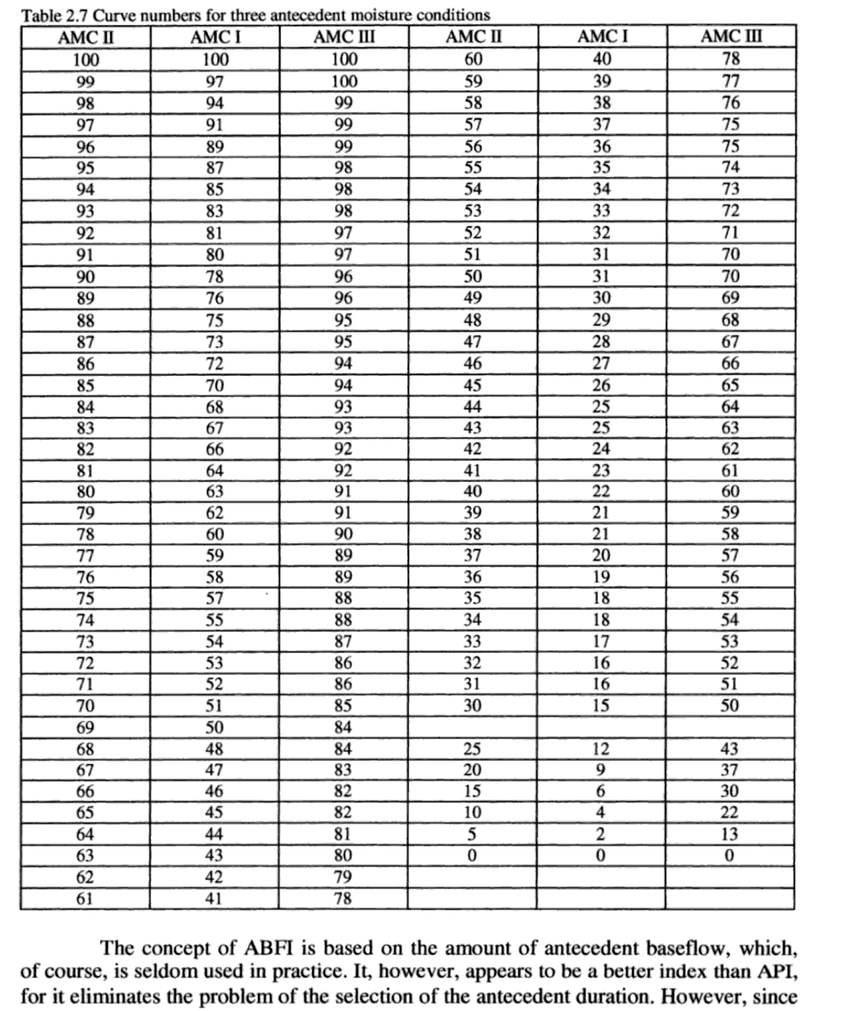
Determination of the soil moisture condition based on 5-day antecedent rainfall totals. The AMC is estimated according to the Soil Conservation Service definitions (SCS, 1986). On top of that the state of the vegetation is a major factor in most events, and included in the strategy here.
Antecedent Soil moisture conditions are based on rainfall amounts and the state of the vegetation (dormant season or not).
AMCclass=pd.read_csv(r"http://vanoproy.be/css/AMC.csv",header=1, sep=",", engine='python', encoding="UTF-8",parse_dates=True );
AMCclass.head()
| AMC class | moisture | Dormant season | Growing season | |
|---|---|---|---|---|
| 0 | AMC I | dry | P<12.7 | P<35.6 |
| 1 | AMC II | medium | 12.7<P<27.9 | 35.6<P<53.3 |
| 2 | AMC III | wet | P>27.9 | P>53.3 |
A dormant season for vegetation is the condition when the month is 11,12,1,2,3. We included the first 20 days of April because the higher elevation means lower mean temperatures, thus a longer winter dormancy can be expected.
Water_Spring_Madonna_di_Canneto["Week"]= Water_Spring_Madonna_di_Canneto.index.isocalendar().week # ["Date"]
Water_Spring_Madonna_di_Canneto["Dormant"]= np.where( (Water_Spring_Madonna_di_Canneto.index.month.isin([11,12,1,2,3])) | (Water_Spring_Madonna_di_Canneto.index.isocalendar().week.isin([15,14,16]) ) ,1,0 ) # add ["1 Apr":"15 Apr"]
Water_Spring_Madonna_di_Canneto["Dormant"].describe()
count 3104.00 mean 0.48 std 0.50 min 0.00 25% 0.00 50% 0.00 75% 1.00 max 1.00 Name: Dormant, dtype: float64
Water_Spring_Madonna_di_Canneto["2014-04-15":"2014-04-21"]#.loc["Dormant"]
| Rainfall_Settefrati | Temperature_Settefrati | Flow_Rate_Madonna_di_Canneto | doy | Month | Week | Dormant | |
|---|---|---|---|---|---|---|---|
| Date | |||||||
| 2014-04-15 | 25.2 | 8.90 | NaN | 105 | 4 | 16 | 1 |
| 2014-04-16 | 3.4 | 6.25 | NaN | 106 | 4 | 16 | 1 |
| 2014-04-17 | 2.6 | 6.05 | NaN | 107 | 4 | 16 | 1 |
| 2014-04-18 | 0.0 | 8.10 | NaN | 108 | 4 | 16 | 1 |
| 2014-04-19 | 13.0 | 7.85 | NaN | 109 | 4 | 16 | 1 |
| 2014-04-20 | 12.6 | 13.05 | NaN | 110 | 4 | 16 | 1 |
| 2014-04-21 | 0.0 | 14.05 | NaN | 111 | 4 | 17 | 0 |
Water_Spring_Madonna_di_Canneto["2015-04-14":"2015-04-21"]#.loc["Dormant"]
| Rainfall_Settefrati | Temperature_Settefrati | Flow_Rate_Madonna_di_Canneto | doy | Month | Week | Dormant | |
|---|---|---|---|---|---|---|---|
| Date | |||||||
| 2015-04-14 | 0.4 | 14.60 | 274.95 | 104 | 4 | 16 | 1 |
| 2015-04-15 | 0.0 | 15.25 | 273.63 | 105 | 4 | 16 | 1 |
| 2015-04-16 | 0.0 | 14.90 | 273.63 | 106 | 4 | 16 | 1 |
| 2015-04-17 | 0.2 | 14.35 | 273.81 | 107 | 4 | 16 | 1 |
| 2015-04-18 | 0.0 | 12.80 | 273.90 | 108 | 4 | 16 | 1 |
| 2015-04-19 | 1.4 | 13.25 | 274.12 | 109 | 4 | 16 | 1 |
| 2015-04-20 | 0.2 | 11.80 | 274.14 | 110 | 4 | 17 | 0 |
| 2015-04-21 | 0.0 | 12.50 | 273.99 | 111 | 4 | 17 | 0 |
Water_Spring_Madonna_di_Canneto[(Water_Spring_Madonna_di_Canneto["Rainfall_Settefrati"].rolling(5).sum()>(27.9)) & (Water_Spring_Madonna_di_Canneto["Dormant"]==1)]
| Rainfall_Settefrati | Temperature_Settefrati | Flow_Rate_Madonna_di_Canneto | doy | Month | Rainfall_5 | Year | Rainfall_Set | Flow_Rate_Mad | TmnStd | Flow_m3_7 | Flow_m3_3 | Flow_m3_22 | Flow_7 | Flow_3 | Flow_22 | Flow_m3_90 | Rainfall_m3_90 | Flow_90 | Rainfall_90 | TmnStd_4 | T_7 | Rainfall_3 | Rainfall_4 | Rainfall_50 | Rainfall_7 | Rainfall_22 | Rainfall_30 | RainCutOff_6 | RainCutOff_5 | RainOvers_6 | CutOff | RainCutOff | RainCutOffmm | RCO_F_cumdif | R_F_cumdif | Dormant | |
|---|---|---|---|---|---|---|---|---|---|---|---|---|---|---|---|---|---|---|---|---|---|---|---|---|---|---|---|---|---|---|---|---|---|---|---|---|---|
| Date | |||||||||||||||||||||||||||||||||||||
| 2015-03-17 | 7.60 | 7.55 | 290.69 | 76 | 3 | 29.4 | 2015 | 51300.0 | 25115.51 | 1.42 | 171405.03 | 75227.64 | 532398.39 | 1983.85 | 870.69 | 6162.02 | 2.14e+06 | 1.61e+06 | 24805.53 | 238.2 | 0.63 | 7.27 | 23.6 | 29.4 | 158.0 | 29.4 | 84.3 | 105.8 | 29.4 | 29.4 | 0.0 | 0 | 7.6 | 2.28e+05 | 7.60e+05 | 76090.98 | 1 |
| 2015-03-18 | 0.00 | 8.40 | 285.42 | 77 | 3 | 29.4 | 2015 | 0.0 | 24660.09 | 2.27 | 171405.03 | 74838.76 | 532398.39 | 1983.85 | 866.19 | 6162.02 | 2.14e+06 | 1.61e+06 | 24805.53 | 238.2 | 0.96 | 7.27 | 16.2 | 23.6 | 158.0 | 29.4 | 84.3 | 105.8 | 29.4 | 29.4 | 0.0 | 0 | 0.0 | 0.00e+00 | 7.35e+05 | 51430.89 | 1 |
| 2015-03-25 | 37.30 | 10.25 | 282.40 | 84 | 3 | 38.1 | 2015 | 251775.0 | 24399.44 | 4.12 | 171516.07 | 73540.03 | 532398.39 | 1985.14 | 851.16 | 6162.02 | 2.14e+06 | 1.61e+06 | 24805.53 | 238.2 | 3.39 | 9.21 | 37.3 | 38.1 | 158.0 | 38.1 | 84.3 | 105.8 | 38.1 | 38.1 | 0.0 | 0 | 37.3 | 1.12e+06 | 1.71e+06 | 137089.82 | 1 |
| 2015-03-26 | 6.00 | 13.35 | 275.94 | 85 | 3 | 44.1 | 2015 | 40500.0 | 23841.00 | 7.22 | 170971.15 | 72792.63 | 532398.39 | 1978.83 | 842.51 | 6162.02 | 2.14e+06 | 1.61e+06 | 24805.53 | 238.2 | 5.09 | 9.73 | 43.3 | 43.3 | 158.0 | 44.1 | 84.3 | 105.8 | 44.1 | 44.1 | 0.0 | 0 | 6.0 | 1.80e+05 | 1.86e+06 | 153748.82 | 1 |
| 2015-03-27 | 10.80 | 12.00 | 273.92 | 86 | 3 | 54.1 | 2015 | 72900.0 | 23666.67 | 5.87 | 170144.30 | 71907.11 | 532398.39 | 1969.26 | 832.26 | 6162.02 | 2.14e+06 | 1.61e+06 | 24805.53 | 238.2 | 5.81 | 10.20 | 54.1 | 54.1 | 158.0 | 54.9 | 84.3 | 105.8 | 54.9 | 54.1 | 0.8 | 0 | 10.8 | 3.24e+05 | 2.16e+06 | 202982.15 | 1 |
| ... | ... | ... | ... | ... | ... | ... | ... | ... | ... | ... | ... | ... | ... | ... | ... | ... | ... | ... | ... | ... | ... | ... | ... | ... | ... | ... | ... | ... | ... | ... | ... | ... | ... | ... | ... | ... | ... |
| 2020-03-08 | 1.76 | NaN | 224.81 | 68 | 3 | 0.0 | 2020 | NaN | 19423.98 | NaN | 135857.20 | 58267.82 | 420393.06 | 1572.42 | 674.40 | 4865.66 | 1.71e+06 | NaN | 19829.03 | NaN | NaN | NaN | NaN | NaN | NaN | NaN | NaN | NaN | NaN | NaN | NaN | 0 | NaN | NaN | NaN | NaN | 1 |
| 2020-03-09 | 1.34 | NaN | 224.79 | 69 | 3 | 0.0 | 2020 | NaN | 19422.08 | NaN | 135906.66 | 58268.74 | 420470.02 | 1572.99 | 674.41 | 4866.55 | 1.71e+06 | NaN | 19833.75 | NaN | NaN | NaN | NaN | NaN | NaN | NaN | NaN | NaN | NaN | NaN | NaN | 0 | NaN | NaN | NaN | NaN | 1 |
| 2020-03-10 | 3.29 | NaN | 224.67 | 70 | 3 | 0.0 | 2020 | NaN | 19411.10 | NaN | 135923.03 | 58257.16 | 420542.18 | 1573.18 | 674.27 | 4867.39 | 1.71e+06 | NaN | 19834.27 | NaN | NaN | NaN | NaN | NaN | NaN | NaN | NaN | NaN | NaN | NaN | NaN | 0 | NaN | NaN | NaN | NaN | 1 |
| 2020-04-05 | 9.64 | NaN | 224.61 | 96 | 4 | 0.0 | 2020 | NaN | 19406.60 | NaN | 135798.90 | 58198.83 | 426837.27 | 1571.75 | 673.60 | 4940.25 | 1.72e+06 | NaN | 19865.32 | NaN | NaN | NaN | NaN | NaN | NaN | NaN | NaN | NaN | NaN | NaN | NaN | 0 | NaN | NaN | NaN | NaN | 1 |
| 2020-04-06 | 1.83 | NaN | 224.50 | 97 | 4 | 0.0 | 2020 | NaN | 19396.86 | NaN | 135798.71 | 58195.41 | 426827.48 | 1571.74 | 673.56 | 4940.13 | 1.72e+06 | NaN | 19866.59 | NaN | NaN | NaN | NaN | NaN | NaN | NaN | NaN | NaN | NaN | NaN | NaN | 0 | NaN | NaN | NaN | NaN | 1 |
173 rows × 37 columns
Water_Spring_Madonna_di_Canneto= Water_Spring_Madonna_di_Canneto.dropna()
pd.set_option('mode.chained_assignment',None)
#Water_Spring_Madonna_di_Canneto= dfW
dfW= Water_Spring_Madonna_di_Canneto
Water_Spring_Madonna_di_Canneto["Rainfall_5"] =Water_Spring_Madonna_di_Canneto["Rainfall_Settefrati"].rolling(5).sum().fillna(0, )#method="bfill"
#Rainfall_5
#dfW=dfW.drop("Rainfall_5")
#dfW.tail()
Water_Spring_Madonna_di_Canneto.tail()
| Rainfall_Settefrati | Temperature_Settefrati | Flow_Rate_Madonna_di_Canneto | doy | Month | Week | Dormant | Rainfall_5 | |
|---|---|---|---|---|---|---|---|---|
| Date | ||||||||
| 2020-06-26 | 1.43 | NaN | 223.92 | 178 | 6 | 26 | 0 | 6.96 |
| 2020-06-27 | 1.50 | NaN | 223.86 | 179 | 6 | 26 | 0 | 6.26 |
| 2020-06-28 | 0.26 | NaN | 223.76 | 180 | 6 | 26 | 0 | 6.06 |
| 2020-06-29 | 0.09 | NaN | 223.77 | 181 | 6 | 27 | 0 | 5.63 |
| 2020-06-30 | 1.84 | NaN | 223.75 | 182 | 6 | 27 | 0 | 5.11 |
Formulations for determination of dry, average and wet vegetation based on the amount of rainfall of previous 5 days.
conditions = [
(Water_Spring_Madonna_di_Canneto["Rainfall_5"]>53.3) & (Water_Spring_Madonna_di_Canneto["Dormant"]==0) ,
(Water_Spring_Madonna_di_Canneto["Rainfall_5"]>27.9) & (Water_Spring_Madonna_di_Canneto["Dormant"]==1),
(Water_Spring_Madonna_di_Canneto["Rainfall_5"]>35.6 ) & (Water_Spring_Madonna_di_Canneto["Dormant"]==0) ,
(Water_Spring_Madonna_di_Canneto["Rainfall_5"]>(27.9)) & (Water_Spring_Madonna_di_Canneto["Dormant"]==1),
(Water_Spring_Madonna_di_Canneto["Rainfall_5"]<=35.6 ) & (Water_Spring_Madonna_di_Canneto["Dormant"]==0) ,
(Water_Spring_Madonna_di_Canneto["Rainfall_5"]<=(27.9)) & (Water_Spring_Madonna_di_Canneto["Dormant"]==1),
]
choices = [2,2,1,1, 0.01,0.01]
Water_Spring_Madonna_di_Canneto['Wet'] = np.select(conditions, choices, default=np.nan)
dfW["Wet"].describe()
dfW["Wet"].plot();

Water_Spring_Madonna_di_Canneto[(Water_Spring_Madonna_di_Canneto["Rainfall_5"]>53.3) & (Water_Spring_Madonna_di_Canneto["Dormant"]==0)]
TR-55: 'Urban Hydrology for Small Watersheds'
Author: USDA Soil Conservation Service (SCS). Now Natural Resources Conservation Service (NRCS)
"Technical Release 55" (TR-55) presents simplified procedures to calculate storm runoff volume, peak rate of discharge, hydrographs, and storage volumes required for floodwater reservoirs. These procedures are applicable to small watersheds, especially urbanizing watersheds, in the United States." Comments:
TR-55 is perhaps the most widely used approach to hydrology in the US. Originally released in 1975, TR-55 provides a number of techniques that are useful for modeling small watersheds. Since the initial publication predated the widespread use of computers, TR-55 was designed primarily as a set of manual worksheets. A TR-55 computer program is now available, based closely on the manual calculations of TR-55.
TR-55 utilizes the SCS runoff equation to predict the peak rate of runoff as well as the total volume. TR-55 also provides a simplified "tabular method" for the generation of complete runoff hydrographs. The tabular method is a simplified technique based on calculations performed with TR-20. TR-55 specifically recommends the use of more precise tools, such as TR-20, if the assumptions of TR-55 are not met.
Recommendations:
While the TR-55 manual remains a most useful reference (it contains complete curve number tables and rainfall maps, among other things) most engineers have sought out more advanced or more accurate hydrology software. How to get it:
You can download the TR-55 Manual here. (2MB PDF format) The complete software and documentation is available from the NRCS TR-55 web page. Also see the NRCS Win-TR-55 web page.
SCS CN- or curve number method
Runoff Equation
The SCS Runoff equation is used with the SCS Unit Hydrograph method to turn rainfall into runoff. It is an empirical method that expresses how much runoff volume is generated by a certain volume of rainfall.
The variable input parameters of the equation are the rainfall amount for a given duration and the basin’s runoff curve number (CN). For convenience, the runoff amount is typically referred to as a runoff volume even though it is expressed in units of depth (in., mm). In fact, this runoff depth is a normalized volume since it is generally distributed over a sub-basin or catchment area.
In hydrograph analysis the SCS runoff equation is applied against an incremental burst of rain to generate a runoff quantity. This runoff quantity is then distributed according to the unit hydrograph procedure, which ultimately develops the full runoff hydrograph.
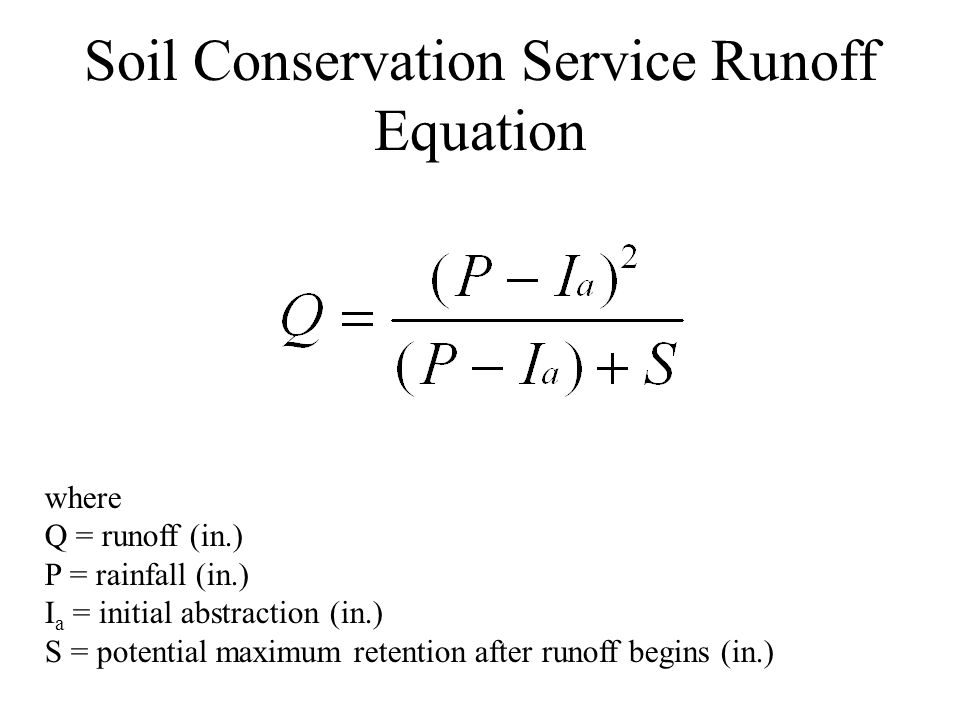
The general form of the equation (U.S. customary units) is:


Q = Runoff depth (in)
P = Rainfall (in)
S = Maximum retention after runoff begins (in), or soil moisture storage deficit
$I_a$ = Initial abstraction
The initial abstraction includes water captured by vegetation, depression storage, evaporation, and infiltration. For any P, this abstraction must be satisfied before any runoff is possible. The universal default for the initial abstraction is given by the equation:
The ratio ${ \lambda }$, 0.2, was rarely modified. Recently, Woodward et al. (2003) analysing event rainfall-runoff data from several hundred plots recommended using $\lambda $=0.05. However, a different ratio ${ \lambda }$ has another CN set, so you have to recalculate S and CN!.
The potential maximum retention after runoff begins, S, is related to the soil and land use/vegetative cover characteristics of the watershed by the equation:
...where the runoff curve number is developed by coincidental tabulation of soil/land use extents in the weighted runoff curve number parameter, CN. CN has a range of 0 to 100.
Alternative for European metric in meter: 
Estimation of surface runoff by curve numbers: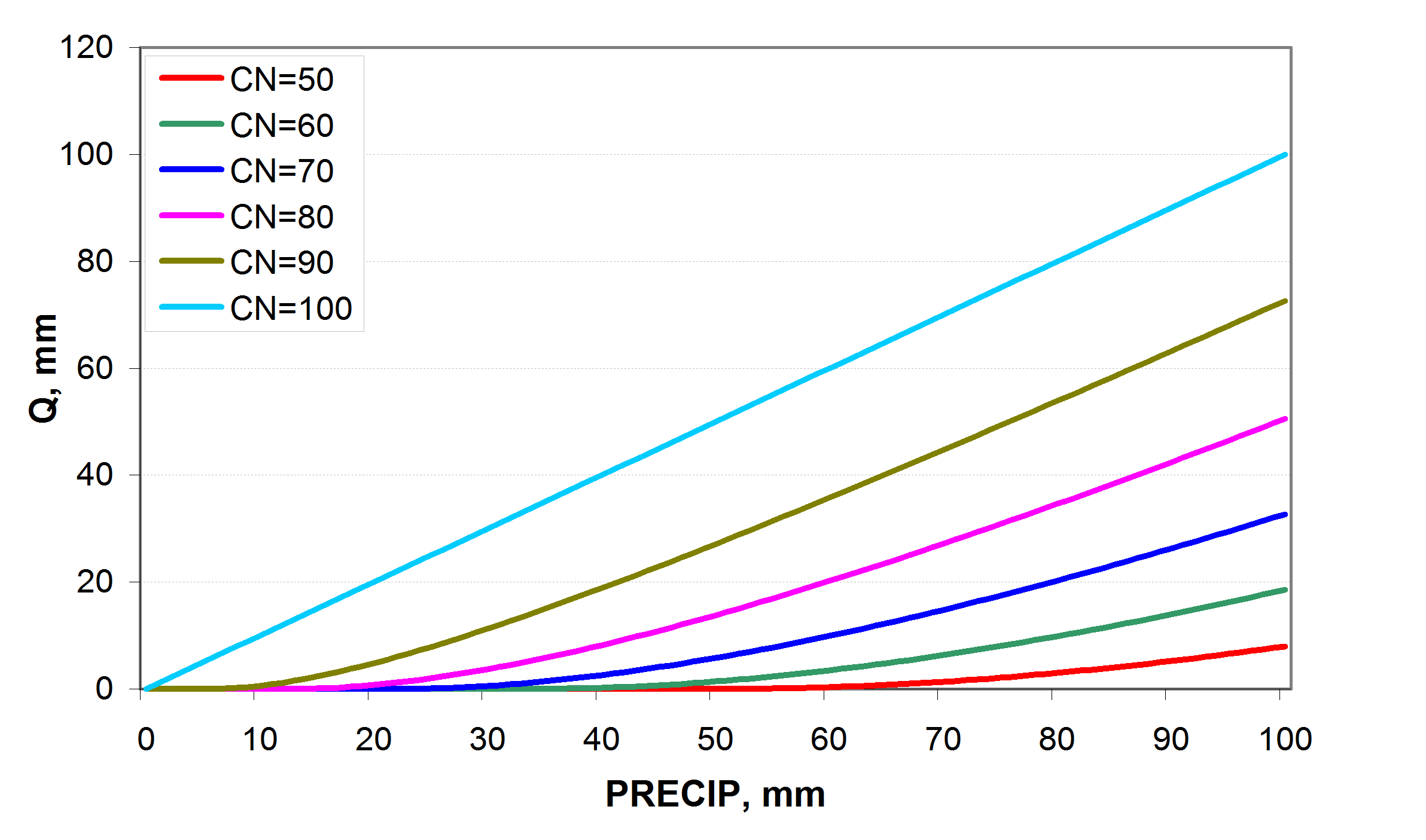
SCS Hydrologic Soil Groups: Soil textures
A. Sand, loamy sand, or sandy loam
B. Silt loam or loam
C. Sandy clay loam
D. Clay loam, silty clay loam, sandy clay, silty clay, or clay
imgInfil

Runoff curve numbers for cultivated/other agricultural lands and soil types
import pandas as pd
CN=pd.read_csv(r"evapotrans/SCS.csv", encoding="UTF-8",engine="python", header=[3]) # header=[2,3] skiprows
CN
| Cover type | Treatment | Hydrologic condition | A | B | C | D | |
|---|---|---|---|---|---|---|---|
| 0 | Fallow | Bare soil | — | 77 | 86 | 91 | 94 |
| 1 | Woods | - | Poor | 45 | 66 | 77 | 83 |
| 2 | Woods | - | Fair | 36 | 60 | 73 | 79 |
| 3 | Woods | - | Good | 30 | 55 | 70 | 77 |
WoodsC= CN.loc[3,"C"]; WoodsD= CN.loc[3,"D"]; BareC= CN.loc[0,"C"]; BareD= CN.loc[0,"D"];
print(WoodsC , WoodsD , BareC , BareD)
70 77 91 94
From soil maps I found that the soil right below the mountainous rocks should be loam, loamy sand or sandy loam. So it must be soil group B, A or mixture.
First we try the coefficients for group B, soil in good condition.
P=30
CN=55
S= (1000/CN)-10
Q = (P- 0.2 *S)**2/(P + 0.8*S) # S is related to the soil and cover conditions of the watershed through the CN.
print(round(Q,4))
22.0136
Calculate runoff depth
It is confusingly called a 'depth', but it is really a volume unit.
Water_Spring_Madonna_di_Canneto.head()
| Rainfall_Settefrati | Temperature_Settefrati | Flow_Rate_Madonna_di_Canneto | doy | Month | Rainfall_5 | Year | Rainfall_Set | Flow_Rate_Mad | TmnStd | Flow_m3_7 | Flow_m3_3 | Flow_m3_22 | Flow_7 | Flow_3 | Flow_22 | Flow_m3_90 | Rainfall_m3_90 | Flow_90 | Rainfall_90 | TmnStd_4 | T_7 | Rainfall_3 | Rainfall_4 | Rainfall_50 | Rainfall_7 | Rainfall_22 | Rainfall_30 | RainCutOff_6 | RainCutOff_5 | RainOvers_6 | CutOff | RainCutOff | RainCutOffmm | RCO_F_cumdif | R_F_cumdif | Dormant | Wet | |
|---|---|---|---|---|---|---|---|---|---|---|---|---|---|---|---|---|---|---|---|---|---|---|---|---|---|---|---|---|---|---|---|---|---|---|---|---|---|---|
| Date | ||||||||||||||||||||||||||||||||||||||
| 2015-03-13 | 0.0 | 5.70 | 255.96 | 72 | 3 | 2.4 | 2015 | 0.0 | 22114.64 | -0.43 | 171405.03 | 72180.35 | 532398.39 | 1983.85 | 835.42 | 6162.02 | 2.14e+06 | 1.61e+06 | 24805.53 | 238.2 | 0.17 | 7.27 | 13.2 | 21.8 | 158.0 | 29.4 | 84.3 | 105.8 | 29.4 | 29.4 | 0.0 | 0 | 0.0 | 0.0 | -22114.64 | -22114.64 | 1 | 0.01 |
| 2015-03-14 | 5.8 | 7.10 | 289.55 | 73 | 3 | 8.2 | 2015 | 39150.0 | 25016.74 | 0.97 | 171405.03 | 72180.35 | 532398.39 | 1983.85 | 835.42 | 6162.02 | 2.14e+06 | 1.61e+06 | 24805.53 | 238.2 | 0.17 | 7.27 | 13.2 | 21.8 | 158.0 | 29.4 | 84.3 | 105.8 | 29.4 | 29.4 | 0.0 | 0 | 5.8 | 174000.0 | 126868.62 | -7981.38 | 1 | 0.01 |
| 2015-03-15 | 7.4 | 4.90 | 289.92 | 74 | 3 | 15.6 | 2015 | 49950.0 | 25048.97 | -1.23 | 171405.03 | 72180.35 | 532398.39 | 1983.85 | 835.42 | 6162.02 | 2.14e+06 | 1.61e+06 | 24805.53 | 238.2 | 0.17 | 7.27 | 13.2 | 21.8 | 158.0 | 29.4 | 84.3 | 105.8 | 29.4 | 29.4 | 0.0 | 0 | 7.4 | 222000.0 | 323819.65 | 16919.65 | 1 | 0.01 |
| 2015-03-16 | 8.6 | 7.50 | 290.08 | 75 | 3 | 24.2 | 2015 | 58050.0 | 25063.16 | 1.37 | 171405.03 | 75128.87 | 532398.39 | 1983.85 | 869.55 | 6162.02 | 2.14e+06 | 1.61e+06 | 24805.53 | 238.2 | 0.17 | 7.27 | 21.8 | 21.8 | 158.0 | 29.4 | 84.3 | 105.8 | 29.4 | 29.4 | 0.0 | 0 | 8.6 | 258000.0 | 556756.49 | 49906.49 | 1 | 0.01 |
| 2015-03-17 | 7.6 | 7.55 | 290.69 | 76 | 3 | 29.4 | 2015 | 51300.0 | 25115.51 | 1.42 | 171405.03 | 75227.64 | 532398.39 | 1983.85 | 870.69 | 6162.02 | 2.14e+06 | 1.61e+06 | 24805.53 | 238.2 | 0.63 | 7.27 | 23.6 | 29.4 | 158.0 | 29.4 | 84.3 | 105.8 | 29.4 | 29.4 | 0.0 | 0 | 7.6 | 228000.0 | 759640.98 | 76090.98 | 1 | 2.00 |
Water_Spring_Madonna_di_Canneto.loc[Water_Spring_Madonna_di_Canneto.Wet == 1]
| Rainfall_Settefrati | Temperature_Settefrati | Flow_Rate_Madonna_di_Canneto | doy | Month | PET | Dormant | Rainfall_5 | Wet | runoffdepth | Infilt | Infiltsum | |
|---|---|---|---|---|---|---|---|---|---|---|---|---|
| Date | ||||||||||||
| 2012-04-23 | 10.00 | 9.80 | NaN | 114.0 | 4.0 | 3.34 | 0.0 | 49.60 | 1.0 | 0.0 | 10.00 | 363.32 |
| 2012-04-24 | 3.60 | 10.80 | NaN | 115.0 | 4.0 | 3.34 | 0.0 | 40.20 | 1.0 | 0.0 | 3.60 | 366.92 |
| 2012-09-14 | 18.00 | 15.00 | NaN | 258.0 | 9.0 | 4.20 | 0.0 | 46.80 | 1.0 | 0.0 | 18.00 | 636.29 |
| 2012-09-15 | 0.00 | 16.00 | NaN | 259.0 | 9.0 | 4.20 | 0.0 | 44.40 | 1.0 | 0.0 | 0.00 | 636.29 |
| 2012-09-16 | 0.00 | 17.35 | NaN | 260.0 | 9.0 | 4.20 | 0.0 | 44.20 | 1.0 | 0.0 | 0.00 | 636.29 |
| ... | ... | ... | ... | ... | ... | ... | ... | ... | ... | ... | ... | ... |
| 2019-09-11 | 12.39 | NaN | 295.89 | 254.0 | 9.0 | 4.20 | 0.0 | 50.43 | 1.0 | 0.0 | 12.39 | 11179.34 |
| 2019-09-12 | 1.07 | NaN | 294.60 | 255.0 | 9.0 | 4.20 | 0.0 | 43.77 | 1.0 | 0.0 | 1.07 | 11180.41 |
| 2019-09-13 | 4.97 | NaN | 295.88 | 256.0 | 9.0 | 4.20 | 0.0 | 48.14 | 1.0 | 0.0 | 4.97 | 11185.38 |
| 2019-09-14 | 6.83 | NaN | NaN | 257.0 | 9.0 | 4.20 | 0.0 | 51.70 | 1.0 | 0.0 | 6.83 | 11192.21 |
| 2019-10-28 | 20.69 | NaN | 218.23 | 301.0 | 10.0 | 2.52 | 0.0 | 49.50 | 1.0 | 0.0 | 20.69 | 11358.61 |
97 rows × 12 columns
The runoff volume / depth is based on dry, average or wet soil condition.
def runoffdepthdry(P):
#print(P)#if W == 0.1: #if dry
CN=35; Q=0
S= (25400/CN)- 254 # (1000/CN)-10 # inches
if P<= 0.2*S:
Q=0
elif P> 0.2*S:
Q = (P- 0.2 *S)**2/(P + 0.8*S) # S is related to the soil and cover conditions of the watershed through the CN.
return Q #round(, 4)
def runoffdepthavg(P):
CN=55; Q=0 # average
S= (25400/CN)- 254 # (1000/CN)-10 # inches
if P<= 0.2*S:
Q=0
elif P> 0.2*S:
Q = (P- 0.2 *S)**2/(P + 0.8*S) # S is related to the soil and cover conditions of the watershed through the CN.
return Q #
def runoffdepthwet(P):
#if wet
CN=74; Q=0
S= (25400/CN)- 254 # (1000/CN)-10 # inches
if P<= 0.2*S:
Q=0
elif P> 0.2*S:
Q = (P- 0.2 *S)**2/(P + 0.8*S) # S is related to the soil and cover conditions of the watershed through the CN.
return Q #
def runoffdepth2(P):
CN=70; Q=0 # ex CN=55
S= (25400/CN)- 254 # in mm retention coefficient
if P<= 0.05*S: Q= 0
elif P> 0.05*S:
Q = (P- 0.05 *S)**2/(P + 0.95*S) # S is related to the soil and cover conditions of the watershed through the CN.
return Q #
# if Water_Spring_Madonna_di_Canneto['Wet'] == 0.1:
droog= Water_Spring_Madonna_di_Canneto.loc[Water_Spring_Madonna_di_Canneto.Wet == 0.01]
Water_Spring_Madonna_di_Canneto['runoffdepth'] = droog.applymap( runoffdepthdry ).loc[:, 'Rainfall_Settefrati'] # in mm
# elif Water_Spring_Madonna_di_Canneto['Wet'] == 1:
medium =Water_Spring_Madonna_di_Canneto.loc[Water_Spring_Madonna_di_Canneto.Wet == 1]
Water_Spring_Madonna_di_Canneto['runoffdepth'] = medium.applymap( runoffdepthavg ).loc[:, 'Rainfall_Settefrati']
# elif Water_Spring_Madonna_di_Canneto['Wet'] == 2:
nat= Water_Spring_Madonna_di_Canneto.loc[Water_Spring_Madonna_di_Canneto.Wet == 2]
Water_Spring_Madonna_di_Canneto['runoffdepth'] = nat.applymap( runoffdepthwet ).loc[:, 'Rainfall_Settefrati']
Water_Spring_Madonna_di_Canneto['runoffdepth']= Water_Spring_Madonna_di_Canneto.runoffdepth.replace( np.nan, 0)
Water_Spring_Madonna_di_Canneto['runoffdepth2'] = Water_Spring_Madonna_di_Canneto.applymap( runoffdepth2 ).loc[:, 'Rainfall_Settefrati']
Water_Spring_Madonna_di_Canneto["Infilt"] =Water_Spring_Madonna_di_Canneto["Rainfall_Settefrati"]-Water_Spring_Madonna_di_Canneto["runoffdepth"]
There is no runoff until the rainwater starts ponding, and this is implemented by the empiric parameter $\lambda$, originally valued at: 0.20, revised value: 0.05. (Hawkings, et ...)
print(round(0.05*((25400/55)- 254),3), round(0.05*((25400/30)- 254),2 ), " S:",round((25400/55)- 254,1 ))
10.391 29.63 S: 207.8
Accounting for forest cover on steep slopes, and rocks or barrow soils that make at least 25% on slopes and on a plateau.
print(round(0.05*((25400/71)- 254),3), round(0.05*((25400/80)- 254),2 ), " S:",round((25400/71)- 254,1 ), "CN combined",55*0.66+93*0.34)
5.187 3.18 S: 103.7 CN combined 67.92
dfW[dfW["Rainfall_Settefrati"] >5.187 ] # ex 10.39
| Rainfall_Settefrati | Temperature_Settefrati | Flow_Rate_Madonna_di_Canneto | doy | Month | date | date_check | Rainfall_5 | |
|---|---|---|---|---|---|---|---|---|
| Date | ||||||||
| 2012-02-01 | 13.8 | 0.40 | NaN | 32 | 2 | 2012-02-01 | 1 days | 16.8 |
| 2012-02-09 | 14.8 | 0.80 | NaN | 40 | 2 | 2012-02-09 | 1 days | 31.2 |
| 2012-02-11 | 10.4 | 0.60 | NaN | 42 | 2 | 2012-02-11 | 1 days | 35.2 |
| 2012-02-12 | 13.2 | 0.25 | NaN | 43 | 2 | 2012-02-12 | 1 days | 47.2 |
| 2012-02-13 | 16.4 | -0.55 | NaN | 44 | 2 | 2012-02-13 | 1 days | 55.8 |
| ... | ... | ... | ... | ... | ... | ... | ... | ... |
| 2018-11-24 | 26.9 | 10.35 | 274.27 | 328 | 11 | 2018-11-24 | 1 days | 99.7 |
| 2018-11-25 | 46.3 | 10.15 | 274.32 | 329 | 11 | 2018-11-25 | 1 days | 74.4 |
| 2018-12-14 | 68.2 | 6.25 | NaN | 348 | 12 | 2018-12-14 | 1 days | 77.8 |
| 2018-12-15 | 23.2 | 3.10 | NaN | 349 | 12 | 2018-12-15 | 1 days | 100.8 |
| 2018-12-17 | 17.8 | 5.20 | NaN | 351 | 12 | 2018-12-17 | 1 days | 120.8 |
354 rows × 8 columns
We have to separate the runoff water, which cannot infiltrate into the soil, from the calculation.
def infiltration(row):
if row["Rainfall_Settefrati"]>= 5.187: # ex 10.39
row["Infilt"] =row["Rainfall_Settefrati"]-row["runoffdepth"]-row["PET"]
elif row["Rainfall_Settefrati"]< 5.187:
row["Infilt"] =row["Rainfall_Settefrati"]-row["PET"] #
return row["Infilt"]
Water_Spring_Madonna_di_Canneto['Infilt'] = Water_Spring_Madonna_di_Canneto.apply(lambda row: infiltration(row), axis=1)
Water_Spring_Madonna_di_Canneto.head() #= Water_Spring_Madonna_di_Canneto.dropna()
| Rainfall_Settefrati | Temperature_Settefrati | Flow_Rate_Madonna_di_Canneto | doy | Month | Week | Dormant | Rainfall_5 | Wet | runoffdepth | PET | PETs | Infilt_ | Infiltsum | Infilt | |
|---|---|---|---|---|---|---|---|---|---|---|---|---|---|---|---|
| Date | |||||||||||||||
| 2012-01-01 | 0.0 | 5.25 | NaN | 1 | 1 | 52 | 1 | 0.0 | 0.01 | 0.0 | 0.91 | 0.91 | -0.91 | -0.91 | -0.91 |
| 2012-01-02 | 5.6 | 6.65 | NaN | 2 | 1 | 1 | 1 | 0.0 | 0.01 | 0.0 | 0.91 | 0.91 | 4.69 | 3.79 | 4.69 |
| 2012-01-03 | 10.0 | 8.85 | NaN | 3 | 1 | 1 | 1 | 0.0 | 0.01 | 0.0 | 0.91 | 0.91 | 9.09 | 12.88 | 9.09 |
| 2012-01-04 | 0.0 | 6.75 | NaN | 4 | 1 | 1 | 1 | 0.0 | 0.01 | 0.0 | 0.91 | 0.91 | -0.91 | 11.98 | -0.91 |
| 2012-01-05 | 1.0 | 5.55 | NaN | 5 | 1 | 1 | 1 | 16.6 | 0.01 | 0.0 | 0.91 | 0.91 | 0.09 | 12.07 | 0.09 |
Water_Spring_Madonna_di_Canneto["Infiltsum"] = Water_Spring_Madonna_di_Canneto["Infilt"].cumsum()
Water_Spring_Madonna_di_Canneto["Infilt2"] =Water_Spring_Madonna_di_Canneto["Rainfall_Settefrati"]-Water_Spring_Madonna_di_Canneto["runoffdepth2"]
Water_Spring_Madonna_di_Canneto["2018"]["Infilt"]#,"Infilt2"
2021-03-11 19:31:23,009 [2736] WARNING py.warnings: <ipython-input-98-860bdca5875b>:1: FutureWarning: Indexing a DataFrame with a datetimelike index using a single string to slice the rows, like `frame[string]`, is deprecated and will be removed in a future version. Use `frame.loc[string]` instead. Water_Spring_Madonna_di_Canneto["2018"]["Infilt"]#,"Infilt2"
Date
2018-01-01 4.29
2018-01-02 4.09
2018-01-03 0.29
2018-01-04 -0.71
2018-01-05 -0.91
...
2018-12-27 -0.89
2018-12-28 -0.89
2018-12-29 -0.89
2018-12-30 -0.89
2018-12-31 -0.89
Name: Infilt, Length: 365, dtype: float64
Water_Spring_Madonna_di_Canneto["runoffdepth"].plot( figsize=(15, 4)); #,"Infilt2"]

Water_Spring_Madonna_di_Canneto["Infilt"].plot( figsize=(15, 4)); #,"Infilt2"]

Before resampling, and convertion of units, and calculate netto in - out, or "rest", we must handle first the other features...
The determination of CN values: by formula method, or by conversion table method
The CN values in normal wetness conditions can be determined through NEH integrated with other conditions, such as land use and hydrologic conditions. The values of other two AMC levels can be obtained, by using conversion tables, or according to the conversion formulas [2] shown as below:
$$CN_1 =(4.2*CN_2 )/( 10- 0.058* CN_2)$$R. in inches!!
$$CN_{3} =( 23*CN_2)/(10 -0.12*CN_2 )$$R. in inches!!
When the CN values are determined, the runoff estimation can be made combined with given rainfall account. $Infiltration=Pr-RO-ET$
CN2=55
#CN1 =( 4.2*CN2)/(10 -(0.058*CN2) ); print("CN1:",round(CN1))
CN1 = CN2/(2.281 -0.01281*CN2) ; print("CN1:",round(CN1), " in meters")
CN1: 35 in meters
CN2=55
#CN3 =( 23*CN2)/(10 -(0.012*CN2) ); print("CN3:",round(CN3))
CN3 = CN2/(0.427 -(0.00573*CN2)) ; print("CN3:",round(CN3), " in meters","the formula fails to produce a meaningfull CN3, so we use the conv. tables")
CN3: 492 in meters the formula fails to produce a meaningfull CN3, so we use the conv. tables
averageTemp2019.info()
<class 'pandas.core.frame.DataFrame'> DatetimeIndex: 365 entries, 2019-01-01 to 2019-12-31 Freq: D Data columns (total 6 columns): # Column Non-Null Count Dtype --- ------ -------------- ----- 0 Rainfall_Settefrati 365 non-null float64 1 Temperature_Settefrati 365 non-null float64 2 Flow_Rate_Madonna_di_Canneto 365 non-null float64 3 doy 365 non-null float64 4 Month 365 non-null int64 5 PET 365 non-null float64 dtypes: float64(5), int64(1) memory usage: 28.1 KB
averageTemp2019
| Rainfall_Settefrati | Temperature_Settefrati | Flow_Rate_Madonna_di_Canneto | doy | Month | PET | |
|---|---|---|---|---|---|---|
| 2019-01-01 | 1.49 | 4.54 | 268.39 | 1.00 | 1 | 0.91 |
| 2019-01-02 | 3.17 | 5.24 | 268.14 | 2.00 | 1 | 0.91 |
| 2019-01-03 | 6.59 | 6.67 | 268.43 | 3.00 | 1 | 0.91 |
| 2019-01-04 | 3.47 | 6.89 | 270.83 | 4.00 | 1 | 0.91 |
| 2019-01-05 | 6.29 | 5.87 | 270.67 | 5.00 | 1 | 0.91 |
| ... | ... | ... | ... | ... | ... | ... |
| 2019-12-27 | 15.26 | 5.96 | 269.19 | 361.25 | 12 | 0.89 |
| 2019-12-28 | 3.29 | 6.19 | 268.90 | 362.25 | 12 | 0.89 |
| 2019-12-29 | 1.51 | 4.71 | 269.00 | 363.25 | 12 | 0.89 |
| 2019-12-30 | 1.49 | 3.54 | 269.14 | 364.25 | 12 | 0.89 |
| 2019-12-31 | 0.11 | 3.94 | 268.76 | 365.25 | 12 | 0.89 |
365 rows × 6 columns
Temperature
this series stops end 2018, and nada from 2019 on... but I could use the averages distilled from the other years
Water_Spring_Madonna_di_Canneto.Temperature_Settefrati.plot(figsize=(20, 3.8));

Water_Spring_Madonna_di_Canneto.update( averageTemp2019["2019-01-01":"2019-12-31"].Temperature_Settefrati) #["2019-01-01":"2019-12-31"]
Water_Spring_Madonna_di_Canneto.update( averageTemp2020["2020-01-01":"2020-12-31"].Temperature_Settefrati)#
Water_Spring_Madonna_di_Canneto["2018-01-01":"2020-12-31"].Temperature_Settefrati.plot();
<AxesSubplot:xlabel='Date'>

Water_Spring_Madonna_di_Canneto.tail() #info()
| Rainfall_Settefrati | Temperature_Settefrati | Flow_Rate_Madonna_di_Canneto | doy | Month | Rainfall_5 | Year | Rainfall_Set | Flow_Rate_Mad | TmnStd | Flow_m3_7 | Flow_m3_3 | Flow_m3_22 | Flow_7 | Flow_3 | Flow_22 | Flow_m3_90 | Rainfall_m3_90 | Flow_90 | ... | Rainfall_4 | Rainfall_50 | Rainfall_7 | Rainfall_22 | Rainfall_30 | RainCutOff_6 | RainCutOff_5 | RainOvers_6 | CutOff | RainCutOff | RainCutOffmm | RCO_F_cumdif | R_F_cumdif | Dormant | Wet | runoffdepth | PET | Infilt | Infiltsum | |
|---|---|---|---|---|---|---|---|---|---|---|---|---|---|---|---|---|---|---|---|---|---|---|---|---|---|---|---|---|---|---|---|---|---|---|---|---|---|---|---|
| Date | |||||||||||||||||||||||||||||||||||||||
| 2020-06-26 | 1.43 | 20.41 | 223.92 | 178 | 6 | 0.0 | 2020 | NaN | 19346.61 | NaN | 135529.14 | 58061.30 | 426305.61 | 1568.62 | 672.01 | 4934.09 | 1.75e+06 | NaN | 20198.06 | ... | NaN | NaN | NaN | NaN | NaN | NaN | NaN | NaN | 0 | NaN | NaN | NaN | NaN | 0 | 0.01 | 0.0 | 6.02 | -4.60 | 328.09 |
| 2020-06-27 | 1.50 | 19.99 | 223.86 | 179 | 6 | 0.0 | 2020 | NaN | 19341.66 | NaN | 135504.96 | 58043.05 | 426311.11 | 1568.34 | 671.79 | 4934.16 | 1.75e+06 | NaN | 20197.33 | ... | NaN | NaN | NaN | NaN | NaN | NaN | NaN | NaN | 0 | NaN | NaN | NaN | NaN | 0 | 0.01 | 0.0 | 6.02 | -4.52 | 323.57 |
| 2020-06-28 | 0.26 | 20.67 | 223.76 | 180 | 6 | 0.0 | 2020 | NaN | 19333.24 | NaN | 135468.81 | 58021.51 | 426260.72 | 1567.93 | 671.55 | 4933.57 | 1.74e+06 | NaN | 20196.59 | ... | NaN | NaN | NaN | NaN | NaN | NaN | NaN | NaN | 0 | NaN | NaN | NaN | NaN | 0 | 0.01 | 0.0 | 6.02 | -5.77 | 317.80 |
| 2020-06-29 | 0.09 | 20.70 | 223.77 | 181 | 6 | 0.0 | 2020 | NaN | 19333.41 | NaN | 135433.90 | 58008.31 | 426191.69 | 1567.52 | 671.39 | 4932.77 | 1.74e+06 | NaN | 20195.81 | ... | NaN | NaN | NaN | NaN | NaN | NaN | NaN | NaN | 0 | NaN | NaN | NaN | NaN | 0 | 0.01 | 0.0 | 6.02 | -5.94 | 311.86 |
| 2020-06-30 | 1.84 | 21.80 | 223.75 | 182 | 6 | 0.0 | 2020 | NaN | 19332.23 | NaN | 135401.84 | 57998.88 | 426128.56 | 1567.15 | 671.28 | 4932.04 | 1.74e+06 | NaN | 20195.05 | ... | NaN | NaN | NaN | NaN | NaN | NaN | NaN | NaN | 0 | NaN | NaN | NaN | NaN | 0 | 0.01 | 0.0 | 6.02 | -4.18 | 307.68 |
5 rows × 42 columns
Flow rate
We'll replace all repeated identical values in column 'Flow_Rate', as I find them doubious, and we'll also replace nan's with 0.
Or shall I drop the duplicates?
- Flow_Rate_Madonna_di_Canneto == 296.6075439
- Flow_Rate_Madonna_di_Canneto == 221.1757507
doubles period 2: 5/11/2016: 19/02/2017
# Drop rows where all data is the same # dfC =
Water_Spring_Madonna_di_Canneto =Water_Spring_Madonna_di_Canneto.drop_duplicates( subset="Flow_Rate_Madonna_di_Canneto", keep='last')#,limit=7
no source water flow means no data, or Nan; but 0 can also mean no running water...
Water_Spring_Madonna_di_Canneto['Flow_Rate_Madonna_di_Canneto']= Water_Spring_Madonna_di_Canneto.Flow_Rate_Madonna_di_Canneto.replace( np.nan, 0)
Water_Spring_Madonna_di_Canneto["2016-04-14"].loc['Flow_Rate_Madonna_di_Canneto']
pd.to_datetime(["2016-04-14":"2016-04-22"]), Water_Spring_Madonna_di_Canneto.Flow_Rate_Madonna_di_Canneto]=0 pd.to_datetime(["2017-02-05":"2017-02-19"]), Water_Spring_Madonna_di_Canneto.Flow_Rate_Madonna_di_Canneto]=0
Conversion of units etc...
Conversion of units: mm/d ->m³/d , and l/s-> m³/d. This way, we obtain a common unit m³, which is usefull to spot numerical mistakes and for a water balance.
Also, the creation of an indicator for the months in order to be able to distinguish the progression of seasons.
The actual drainage area for the source is not given, and is probably unknown. I'll give here an estimation based on my study of the topology of the place. I imagined from where higher up any water could trickle down and reach the water spring.
Update 15/5/2022:
I found a map about the aquifers and subterrain water resources of the parc Abruzzo. It features an outline for the drainage area S. capodaqua Val Canneto. A rough calculation of the surface area is 22-23 km².
pd.set_option('mode.chained_assignment',None)
Water_Spring_Madonna_di_Canneto["Month"] =Water_Spring_Madonna_di_Canneto.index.month
Water_Spring_Madonna_di_Canneto["Year"] =Water_Spring_Madonna_di_Canneto.index.year
Water_Spring_Madonna_di_Canneto["Rainfall_Set"] =Water_Spring_Madonna_di_Canneto.Rainfall_Settefrati* 22 *1000*1000/ 1000 # ex 4.5*1.5
Water_Spring_Madonna_di_Canneto["Flow_Rate_Mad"]= Water_Spring_Madonna_di_Canneto.Flow_Rate_Madonna_di_Canneto*24*3600 /1000 #
Water_Spring_Madonna_di_Canneto.info() # no duplicates
<class 'pandas.core.frame.DataFrame'> DatetimeIndex: 1277 entries, 2015-03-13 to 2020-06-30 Data columns (total 11 columns): # Column Non-Null Count Dtype --- ------ -------------- ----- 0 Rainfall_Settefrati 768 non-null float64 1 Temperature_Settefrati 768 non-null float64 2 Flow_Rate_Madonna_di_Canneto 1277 non-null float64 3 doy 1277 non-null int64 4 Month 1277 non-null int64 5 date 1277 non-null datetime64[ns] 6 date_check 1277 non-null timedelta64[ns] 7 Rainfall_5 1277 non-null float64 8 Year 1277 non-null int64 9 Rainfall_Set 768 non-null float64 10 Flow_Rate_Mad 1277 non-null float64 dtypes: datetime64[ns](1), float64(6), int64(3), timedelta64[ns](1) memory usage: 119.7 KB
Water_Spring_Madonna_di_Canneto.head() # no duplicates
| Rainfall_Settefrati | Temperature_Settefrati | Flow_Rate_Madonna_di_Canneto | doy | Month | PET | Dormant | Rainfall_5 | Wet | runoffdepth | Infilt | Infiltsum | |
|---|---|---|---|---|---|---|---|---|---|---|---|---|
| Date | ||||||||||||
| 2012-01-01 00:00:00 | 0.0 | 5.25 | NaN | 1.0 | 1.0 | 0.91 | 1.0 | 0.0 | 0.01 | 0.0 | 0.0 | 0.0 |
| 2012-01-02 00:00:00 | 5.6 | 6.65 | NaN | 2.0 | 1.0 | 0.91 | 1.0 | 0.0 | 0.01 | 0.0 | 5.6 | 5.6 |
| 2012-01-03 00:00:00 | 10.0 | 8.85 | NaN | 3.0 | 1.0 | 0.91 | 1.0 | 0.0 | 0.01 | 0.0 | 10.0 | 15.6 |
| 2012-01-04 00:00:00 | 0.0 | 6.75 | NaN | 4.0 | 1.0 | 0.91 | 1.0 | 0.0 | 0.01 | 0.0 | 0.0 | 15.6 |
| 2012-01-05 00:00:00 | 1.0 | 5.55 | NaN | 5.0 | 1.0 | 0.91 | 1.0 | 16.6 | 0.01 | 0.0 | 1.0 | 16.6 |
%precision 4
2500*750
1875000
print("Flow rates: Minimum:", Water_Spring_Madonna_di_Canneto.iloc[:,2].min(), "Average:", Water_Spring_Madonna_di_Canneto.iloc[:,2].mean(), "Maximum:", Water_Spring_Madonna_di_Canneto.iloc[:,2].max(),"St.d.:",
Water_Spring_Madonna_di_Canneto.iloc[:,2].std(),"Variation:", Water_Spring_Madonna_di_Canneto.iloc[:,2].var())
Flow rates: Minimum: 0.0 Average: 260.4125854539546 Maximum: 300.1609827 St.d.: 32.624516081381806 Variation: 1064.3590495443402
Water_Spring_Madonna_di_Canneto.describe().T # no duplicates
| count | mean | std | min | 25% | 50% | 75% | max | |
|---|---|---|---|---|---|---|---|---|
| Rainfall_Settefrati | 764.0 | 4.17 | 11.90 | 0.00e+00 | 0.00e+00 | 0.00e+00 | 2.42 | 140.80 |
| Temperature_Settefrati | 764.0 | 15.19 | 6.11 | 5.50e-01 | 1.07e+01 | 1.52e+01 | 19.95 | 31.10 |
| Flow_Rate_Madonna_di_Canneto | 764.0 | 276.62 | 23.44 | 1.88e+02 | 2.75e+02 | 2.85e+02 | 290.60 | 300.16 |
| doy | 764.0 | 198.74 | 90.32 | 1.00e+00 | 1.26e+02 | 2.03e+02 | 275.25 | 365.00 |
| Month | 764.0 | 7.03 | 2.97 | 1.00e+00 | 5.00e+00 | 7.00e+00 | 10.00 | 12.00 |
| PET | 764.0 | 3.92 | 2.16 | 8.95e-01 | 2.04e+00 | 4.20e+00 | 6.02 | 7.52 |
| Dormant | 764.0 | 0.33 | 0.47 | 0.00e+00 | 0.00e+00 | 0.00e+00 | 1.00 | 1.00 |
| Rainfall_5 | 764.0 | 20.99 | 35.87 | -7.11e-15 | 1.40e+00 | 1.02e+01 | 25.40 | 359.60 |
| Flag1 | 764.0 | 0.33 | 0.70 | 1.00e-02 | 1.00e-02 | 1.00e-02 | 0.01 | 2.00 |
| Wet | 764.0 | 0.33 | 0.70 | 1.00e-02 | 1.00e-02 | 1.00e-02 | 0.01 | 2.00 |
| Flow_7 | 764.0 | 1936.59 | 156.19 | 1.35e+03 | 1.92e+03 | 1.99e+03 | 2032.53 | 2083.16 |
| Flow_3 | 764.0 | 829.92 | 69.01 | 5.67e+02 | 8.24e+02 | 8.53e+02 | 871.33 | 900.10 |
| Flow_22 | 764.0 | 6086.74 | 433.35 | 4.44e+03 | 6.03e+03 | 6.23e+03 | 6361.22 | 6491.86 |
| RainCutOff_5 | 764.0 | 20.87 | 35.61 | -1.07e-14 | 1.40e+00 | 1.02e+01 | 25.40 | 359.60 |
| RainCutOff_6 | 764.0 | 25.06 | 39.64 | 0.00e+00 | 2.80e+00 | 1.24e+01 | 31.42 | 360.00 |
| RainOvers_6 | 764.0 | 4.18 | 11.90 | -1.42e-14 | 7.11e-15 | 1.42e-14 | 2.60 | 140.80 |
| CutOff | 764.0 | 0.11 | 0.32 | 0.00e+00 | 0.00e+00 | 0.00e+00 | 0.00 | 1.00 |
| RainCutOff | 764.0 | 2.44 | 5.74 | 0.00e+00 | 0.00e+00 | 0.00e+00 | 1.60 | 47.40 |
Water_Spring_Madonna_di_Canneto.to_csv("Madonna_di_Canneto_PET.csv" )
Here, I create a column to simulate a minimum temperature.
Water_Spring_Madonna_di_Canneto.Temperature_Settefrati.std(skipna=True)
6.130628847926524
Water_Spring_Madonna_di_Canneto["TmnStd"] =Water_Spring_Madonna_di_Canneto.Temperature_Settefrati- Water_Spring_Madonna_di_Canneto.Temperature_Settefrati.std(skipna=True)
Water_Spring_Madonna_di_Canneto=pd.read_csv("Madonna_di_Canneto_PET.csv", parse_dates=["Date"],index_col=0 ); Water_Spring_Madonna_di_Canneto
| Rainfall_Settefrati | Temperature_Settefrati | Flow_Rate_Madonna_di_Canneto | doy | Month | Rainfall_5 | Year | Rainfall_Set | Flow_Rate_Mad | TmnStd | Flow_m3_7 | Flow_m3_3 | Flow_m3_22 | Flow_7 | Flow_3 | Flow_22 | Flow_m3_90 | Rainfall_m3_90 | Flow_90 | ... | Rainfall_4 | Rainfall_50 | Rainfall_7 | Rainfall_22 | Rainfall_30 | RainCutOff_6 | RainCutOff_5 | RainOvers_6 | CutOff | RainCutOff | RainCutOffmm | RCO_F_cumdif | R_F_cumdif | Dormant | Wet | runoffdepth | PET | Infilt | Infiltsum | |
|---|---|---|---|---|---|---|---|---|---|---|---|---|---|---|---|---|---|---|---|---|---|---|---|---|---|---|---|---|---|---|---|---|---|---|---|---|---|---|---|
| Date | |||||||||||||||||||||||||||||||||||||||
| 2015-03-13 | 0.00 | 5.70 | 255.96 | 72 | 3 | 2.4 | 2015 | 0.0 | 22114.64 | -0.43 | 171405.03 | 72180.35 | 532398.39 | 1983.85 | 835.42 | 6162.02 | 2.14e+06 | 1.61e+06 | 24805.53 | ... | 21.8 | 158.0 | 29.4 | 84.3 | 105.8 | 29.4 | 29.4 | 0.0 | 0 | 0.0 | 0.0 | -22114.64 | -22114.64 | 1 | 0.01 | 0.0 | 2.04 | -2.04 | -2.04 |
| 2015-03-14 | 5.80 | 7.10 | 289.55 | 73 | 3 | 8.2 | 2015 | 39150.0 | 25016.74 | 0.97 | 171405.03 | 72180.35 | 532398.39 | 1983.85 | 835.42 | 6162.02 | 2.14e+06 | 1.61e+06 | 24805.53 | ... | 21.8 | 158.0 | 29.4 | 84.3 | 105.8 | 29.4 | 29.4 | 0.0 | 0 | 5.8 | 174000.0 | 126868.62 | -7981.38 | 1 | 0.01 | 0.0 | 2.04 | 3.76 | 1.72 |
| 2015-03-15 | 7.40 | 4.90 | 289.92 | 74 | 3 | 15.6 | 2015 | 49950.0 | 25048.97 | -1.23 | 171405.03 | 72180.35 | 532398.39 | 1983.85 | 835.42 | 6162.02 | 2.14e+06 | 1.61e+06 | 24805.53 | ... | 21.8 | 158.0 | 29.4 | 84.3 | 105.8 | 29.4 | 29.4 | 0.0 | 0 | 7.4 | 222000.0 | 323819.65 | 16919.65 | 1 | 0.01 | 0.0 | 2.04 | 5.36 | 7.08 |
| 2015-03-16 | 8.60 | 7.50 | 290.08 | 75 | 3 | 24.2 | 2015 | 58050.0 | 25063.16 | 1.37 | 171405.03 | 75128.87 | 532398.39 | 1983.85 | 869.55 | 6162.02 | 2.14e+06 | 1.61e+06 | 24805.53 | ... | 21.8 | 158.0 | 29.4 | 84.3 | 105.8 | 29.4 | 29.4 | 0.0 | 0 | 8.6 | 258000.0 | 556756.49 | 49906.49 | 1 | 0.01 | 0.0 | 2.04 | 6.56 | 13.64 |
| 2015-03-17 | 7.60 | 7.55 | 290.69 | 76 | 3 | 29.4 | 2015 | 51300.0 | 25115.51 | 1.42 | 171405.03 | 75227.64 | 532398.39 | 1983.85 | 870.69 | 6162.02 | 2.14e+06 | 1.61e+06 | 24805.53 | ... | 29.4 | 158.0 | 29.4 | 84.3 | 105.8 | 29.4 | 29.4 | 0.0 | 0 | 7.6 | 228000.0 | 759640.98 | 76090.98 | 1 | 2.00 | 0.0 | 2.04 | 5.56 | 19.19 |
| ... | ... | ... | ... | ... | ... | ... | ... | ... | ... | ... | ... | ... | ... | ... | ... | ... | ... | ... | ... | ... | ... | ... | ... | ... | ... | ... | ... | ... | ... | ... | ... | ... | ... | ... | ... | ... | ... | ... | ... |
| 2020-06-26 | 1.43 | 20.41 | 223.92 | 178 | 6 | 0.0 | 2020 | NaN | 19346.61 | NaN | 135529.14 | 58061.30 | 426305.61 | 1568.62 | 672.01 | 4934.09 | 1.75e+06 | NaN | 20198.06 | ... | NaN | NaN | NaN | NaN | NaN | NaN | NaN | NaN | 0 | NaN | NaN | NaN | NaN | 0 | 0.01 | 0.0 | 6.02 | -4.60 | 328.09 |
| 2020-06-27 | 1.50 | 19.99 | 223.86 | 179 | 6 | 0.0 | 2020 | NaN | 19341.66 | NaN | 135504.96 | 58043.05 | 426311.11 | 1568.34 | 671.79 | 4934.16 | 1.75e+06 | NaN | 20197.33 | ... | NaN | NaN | NaN | NaN | NaN | NaN | NaN | NaN | 0 | NaN | NaN | NaN | NaN | 0 | 0.01 | 0.0 | 6.02 | -4.52 | 323.57 |
| 2020-06-28 | 0.26 | 20.67 | 223.76 | 180 | 6 | 0.0 | 2020 | NaN | 19333.24 | NaN | 135468.81 | 58021.51 | 426260.72 | 1567.93 | 671.55 | 4933.57 | 1.74e+06 | NaN | 20196.59 | ... | NaN | NaN | NaN | NaN | NaN | NaN | NaN | NaN | 0 | NaN | NaN | NaN | NaN | 0 | 0.01 | 0.0 | 6.02 | -5.77 | 317.80 |
| 2020-06-29 | 0.09 | 20.70 | 223.77 | 181 | 6 | 0.0 | 2020 | NaN | 19333.41 | NaN | 135433.90 | 58008.31 | 426191.69 | 1567.52 | 671.39 | 4932.77 | 1.74e+06 | NaN | 20195.81 | ... | NaN | NaN | NaN | NaN | NaN | NaN | NaN | NaN | 0 | NaN | NaN | NaN | NaN | 0 | 0.01 | 0.0 | 6.02 | -5.94 | 311.86 |
| 2020-06-30 | 1.84 | 21.80 | 223.75 | 182 | 6 | 0.0 | 2020 | NaN | 19332.23 | NaN | 135401.84 | 57998.88 | 426128.56 | 1567.15 | 671.28 | 4932.04 | 1.74e+06 | NaN | 20195.05 | ... | NaN | NaN | NaN | NaN | NaN | NaN | NaN | NaN | 0 | NaN | NaN | NaN | NaN | 0 | 0.01 | 0.0 | 6.02 | -4.18 | 307.68 |
1277 rows × 42 columns
correction for drainage area 22 km²
Water_Spring_Madonna_di_Canneto["Rainfall_Set"] =Water_Spring_Madonna_di_Canneto.Rainfall_Settefrati* 22 *1000*1000/ 1000 # ex 4.5*1.5
Water_Spring_Madonna_di_Canneto["Rainfall_m3_90"] =Water_Spring_Madonna_di_Canneto.Rainfall_Set.rolling(90).sum().fillna( method ='bfill', limit =90)
Yearly and monthly aggregates
CannetoRainyear =Water_Spring_Madonna_di_Canneto.Rainfall_Set.resample('YS').sum();
CannetoRainmonth =Water_Spring_Madonna_di_Canneto.Rainfall_Set.resample('MS').sum();
CannetoRainyearmm =Water_Spring_Madonna_di_Canneto.Rainfall_Settefrati.resample('YS').sum(); CannetoRainyearmm
Date 2015-01-01 280.00 2016-01-01 656.90 2017-01-01 1252.60 2018-01-01 1014.90 2019-01-01 1365.03 2020-01-01 771.61 Freq: AS-JAN, Name: Rainfall_Settefrati, dtype: float64
CannetoRainmonthdf = CannetoRainmonth.to_frame()
fig, ax=plt.subplots(1,1, figsize=(20, 5)); sns.barplot(x=CannetoRainmonthdf.index ,y=CannetoRainmonthdf.Rainfall_Set, data=CannetoRainmonthdf.loc["2012":"2018"]); #
#ax.xlabel(rotation=60);

CannetoFlowmonth =Water_Spring_Madonna_di_Canneto.Flow_Rate_Mad.resample('MS').mean()
CannetoFlowyear = Water_Spring_Madonna_di_Canneto.Flow_Rate_Mad.resample('YS').sum(); #CannetoFlowyear
CannetoFlowyear
Date 2015-01-01 2.26e+06 2016-01-01 4.79e+06 2017-01-01 7.33e+06 2018-01-01 3.98e+06 2019-01-01 6.95e+06 2020-01-01 3.42e+06 Freq: AS-JAN, Name: Flow_Rate_Mad, dtype: float64
CannetoRainyear
Date 2015-01-01 6.16e+06 2016-01-01 1.45e+07 2017-01-01 2.76e+07 2018-01-01 2.23e+07 2019-01-01 3.00e+07 2020-01-01 1.70e+07 Freq: AS-JAN, Name: Rainfall_Set, dtype: float64
sns.barplot(x=CannetoRainyear.index.year, y=CannetoRainyear, data=CannetoRainyear["2013":"2019"]);

sns.barplot(x=CannetoFlowyear.index.year, y=CannetoFlowyear, data=CannetoFlowyear["2013":"2019"] );

22500*3600*24/1000 # *365
1944000.0
1255/1000*50000000 # *365
62750000.0000
Flow rate is on average 300 000 m³ annually. The amount of rainfall in Settefrati: 2-8 000 000 m³, which is 5 km away from the source Madonna di Canneto.
There should be a point where excess rain cannot infiltrate anymore, and just runs off. But this depends on dry, medium or wet soil condition.
CannetoFlowmonth = Water_Spring_Madonna_di_Canneto["2015-01-01":"2020-04-01"].Flow_Rate_Mad.resample('MS').sum();
#CannetoFlowweek = Water_Spring_Madonna_di_Canneto["2015-01-01":"2020-04-01"].Flow_Rate_Mad.resample('W').sum();
CannetoRainmonth = Water_Spring_Madonna_di_Canneto["2015-01-01":"2020-04-01"].Rainfall_Set.resample('MS').sum();
#CannetoRainweek = Water_Spring_Madonna_di_Canneto["2015-01-01":"2020-04-01"].Rainfall_Set.resample('W').sum();
CannetoTempmonth = Water_Spring_Madonna_di_Canneto["2015-01-01":"2020-04-01"].TmnStd.resample('MS').mean();
fig, ax = plt.subplots(2,1, figsize=(20, 5.8), sharex=True) ; plt.title("Rainfall in m³")
sns.lineplot( data=CannetoTempmonth , ax=ax[0])
sns.lineplot( data=CannetoRainmonth, ax=ax[1] )
sns.lineplot( data= CannetoFlowmonth, ax=ax[1] );

Flow rate monthly in l/s.
CannetoFlow_Ratemonth = Water_Spring_Madonna_di_Canneto["2015-01-01":"2020-04-01"].groupby(["Year",'Month'])[["Flow_Rate_Madonna_di_Canneto"]].mean();
CannetoFlow_Ratemonth.plot( figsize=(20, 4));

Flow_Ratemonthno0 =Water_Spring_Madonna_di_Canneto[Water_Spring_Madonna_di_Canneto.Flow_Rate_Madonna_di_Canneto!= 0]
CannetoFlow_Ratemonthno0= Flow_Ratemonthno0["2015-01-01":"2020-04-01"].groupby('Month')[["Flow_Rate_Madonna_di_Canneto"]].mean();
CannetoFlow_Ratemonthno0.plot(figsize=(20, 4));

"2015-03-11":"2019" start / end of Flow rate data
dfC= Water_Spring_Madonna_di_Canneto["2015":"2020"] # > quake plot
Madonna_di_Canneto =dfC["2015-01-01":"2020"] # Water_Spring_Madonna_di_Canneto["2015":"2019"]
Madonna_di_Canneto["2016-04-14":"2016-04-22"] # doubles period 1
| Rainfall_Settefrati | Temperature_Settefrati | Flow_Rate_Madonna_di_Canneto | doy | Month | Rainfall_5 | Year | Rainfall_Set | Flow_Rate_Mad | TmnStd | |
|---|---|---|---|---|---|---|---|---|---|---|
| Date | ||||||||||
| 2016-04-22 | 0.0 | 12.6 | 221.18 | 113 | 4 | 7.11e-15 | 2016 | 0.0 | 19109.58 | 6.47 |
fig, ax = plt.subplots(1,2, figsize=(18, 4), ) # sharey=True
sns.kdeplot(data= Water_Spring_Madonna_di_Canneto.iloc[:,2] ,cut=185, bw_adjust=0.1, ax=ax[0]);
sns.kdeplot(data= Water_Spring_Madonna_di_Canneto.iloc[:,0] ,cut=0, bw_adjust=1, ax=ax[1]); #plt.xlim( 185,300);

fig, ax = plt.subplots(1,2, figsize=(18, 4), ) # - duplicates
sns.kdeplot(data= Madonna_di_Canneto.Flow_Rate_Mad ,cut=185, bw_adjust=0.1, ax=ax[0]);
sns.kdeplot(data= Madonna_di_Canneto.iloc[:,1] , bw_adjust=1, ax=ax[1]); #plt.xlim( 185,300);

Madonna_di_Canneto.Flow_Rate_Mad.plot( kind="hist",bins=20);

The histogram shows us there are 2 regimes in this system to give a combined effect on outflow. Perhaps there are 2 compartments, parallel or on top of each other. We make an extra column to indicate when the total sum of 11 days rain fall > 60-105: from "level 1" to "level 2".
More considerations after several observations:
- In 2017 the water flow increased strongly after there has been torrential rainfall. In September the amount of 140 liters/m² could bring the flow rate back up to almost the maximum value. This jump appeared to happen in 3 times: a first wave after 2 days, and a second and third wave after 4-5 days.
- The flow rate might follow an exponential decay.
- The infiltration area situated 'before' the waterpool is roughly 24 km². But this is likely not a part of the Madonna area.
After a deeper look at the flow rate, I noted:
- From 13 to 22/4/16 all flow rates have the same value. This is also the case from 5/2 to 19/2/2017.
- This is odd, and I don't know this is an human error, or a correction to insert some average data points.
- this manipulates the sample mean, so I think to remove them, or reduce it to a single value, or use discharge coefficient...
- 2 remarkable deep dives in the flow rate: 27/3/17 and 15/11/2018.
- the first can be due to an earthquake with mag. 2.8 that day
- for 15/11/2018 I managed to find that an earthquake occured nearby with mag. 2.5 at 41.68 N 12.76 E. so we'll have to tolerate them, or make the spikes smooth
Check if duplicates have been removed:
Water_Spring_Madonna_di_Canneto.iloc[1563:1578,:]
| Rainfall_Settefrati | Temperature_Settefrati | Flow_Rate_Madonna_di_Canneto | doy | Month | Rainfall_5 | Year | Rainfall_Set | Flow_Rate_Mad | TmnStd | |
|---|---|---|---|---|---|---|---|---|---|---|
| Date |
Water_Spring_Madonna_di_Canneto.iloc[1769:1878,:]
| Rainfall_Settefrati | Temperature_Settefrati | Flow_Rate_Madonna_di_Canneto | Dormant | Wet | runoffdepth | Infilt | Avg | Dry | Month | Year | Rainfall_Set | Flow_Rate_Mad | TmnStd | p | 𝐸𝑇𝑜 | |
|---|---|---|---|---|---|---|---|---|---|---|---|---|---|---|---|---|
| Date |
Water_Spring_Madonna_di_Canneto.iloc[2549:2578,:]
Madonna_di_Canneto =dfC["2015-01-01":"2020"] # Water_Spring_Madonna_di_Canneto["2015":"2019"]
%precision 4
print(226.2879-201.074, 277.0259-226.2879, 277.0259-201.074, 295.192-277.0259, 295.192-201.074)
Rolling sums
Add columns with a rainfall rolling sum of 2, 4, 30 and 6 days. Also we make rolling sums of 2, 7, 50, 60 and 42 days for the temperature and the flow rate.
Water_Spring_Madonna_di_Canneto["Flow_m3_7"] =Water_Spring_Madonna_di_Canneto.Flow_Rate_Mad.rolling(7).sum().fillna( method ='bfill', limit =7) # Flow_Rate_Madonna_di_Canneto
Water_Spring_Madonna_di_Canneto["Flow_m3_3"] =Water_Spring_Madonna_di_Canneto.Flow_Rate_Mad.rolling(3).sum().fillna( method ='bfill', limit =3)
Water_Spring_Madonna_di_Canneto["Flow_m3_22"] =Water_Spring_Madonna_di_Canneto.Flow_Rate_Mad.rolling(22).sum().fillna( method ='bfill', limit =22)
Water_Spring_Madonna_di_Canneto["Flow_7"] =Water_Spring_Madonna_di_Canneto.Flow_Rate_Madonna_di_Canneto.rolling(7).sum().fillna( method ='bfill', limit =7) # Flow_Rate_Madonna_di_Canneto
Water_Spring_Madonna_di_Canneto["Flow_3"] =Water_Spring_Madonna_di_Canneto.Flow_Rate_Madonna_di_Canneto.rolling(3).sum().fillna( method ='bfill', limit =3)
Water_Spring_Madonna_di_Canneto["Flow_22"] =Water_Spring_Madonna_di_Canneto.Flow_Rate_Madonna_di_Canneto.rolling(22).sum().fillna( method ='bfill', limit =22)
Water_Spring_Madonna_di_Canneto["Flow_m3_90"] =Water_Spring_Madonna_di_Canneto.Flow_Rate_Mad.rolling(90).sum().fillna( method ='bfill', limit =90)
Water_Spring_Madonna_di_Canneto["Rainfall_m3_90"] =Water_Spring_Madonna_di_Canneto.Rainfall_Set.rolling(90).sum().fillna( method ='bfill', limit =90)
Water_Spring_Madonna_di_Canneto["Flow_90"] =Water_Spring_Madonna_di_Canneto.Flow_Rate_Madonna_di_Canneto.rolling(90).sum().fillna( method ='bfill', limit =90)
Water_Spring_Madonna_di_Canneto["Rainfall_90"] =Water_Spring_Madonna_di_Canneto.Rainfall_Settefrati.rolling(90).sum().fillna( method ='bfill', limit =90)
Add some temperature means, and subtract the standard deviation in order to simulate a minimum temperature behaviour.
#Water_Spring_Madonna_di_Canneto["T_3"] =Water_Spring_Madonna_di_Canneto.TmnStd.rolling(3).mean()
Water_Spring_Madonna_di_Canneto["TmnStd_4"] =Water_Spring_Madonna_di_Canneto.TmnStd.rolling(4).mean().fillna(method ='bfill', limit =4)
Water_Spring_Madonna_di_Canneto["T_7"] =Water_Spring_Madonna_di_Canneto.Temperature_Settefrati.rolling(7).mean().fillna(method ='bfill', limit = 7) # baseline
#Water_Spring_Madonna_di_Canneto
Water_Spring_Madonna_di_Canneto["Rainfall_3"] =Water_Spring_Madonna_di_Canneto.Rainfall_Settefrati.rolling(3).sum().fillna(method ='bfill', limit = 3)
Water_Spring_Madonna_di_Canneto["Rainfall_4"] =Water_Spring_Madonna_di_Canneto.Rainfall_Settefrati.rolling(4).sum().fillna(method ='bfill', limit = 4)
Water_Spring_Madonna_di_Canneto["Rainfall_50"] =Water_Spring_Madonna_di_Canneto.Rainfall_Settefrati.rolling(50).sum().fillna(method ='bfill', limit = 50)
#Water_Spring_Madonna_di_Canneto["Rainfall_60"] =Water_Spring_Madonna_di_Canneto.Rainfall_Settefrati.rolling(60).sum().fillna('bfill')
Water_Spring_Madonna_di_Canneto["Rainfall_7"] =Water_Spring_Madonna_di_Canneto.Rainfall_Settefrati.rolling(7).sum().fillna(method ='bfill', limit = 7)
Water_Spring_Madonna_di_Canneto["Rainfall_22"] =Water_Spring_Madonna_di_Canneto.Rainfall_Settefrati.rolling(22).sum().fillna(method ='bfill', limit =22)
Water_Spring_Madonna_di_Canneto["Rainfall_30"] =Water_Spring_Madonna_di_Canneto.Rainfall_Settefrati.rolling(30).sum().fillna(method ='bfill', limit =30)
We make a 5 day moving sum for placing a limit on the amount of rainfall that can infiltrate due to soil saturation, with cut off at 55 mm.
Water_Spring_Madonna_di_Canneto[Water_Spring_Madonna_di_Canneto.Rainfall_Settefrati.rolling(5).sum().fillna(method ='bfill', limit = 5)>55]
| Rainfall_Settefrati | Temperature_Settefrati | Flow_Rate_Madonna_di_Canneto | doy | Month | PET | Dormant | Rainfall_5 | Flag1 | Wet | Flow_7 | Flow_3 | Flow_22 | |
|---|---|---|---|---|---|---|---|---|---|---|---|---|---|
| Date | |||||||||||||
| 2016-04-24 | 32.5 | 9.30 | 275.67 | 115.0 | 4.0 | 3.34 | 1.0 | 58.3 | 2.0 | 2.0 | 1638.20 | 737.43 | 5699.11 |
| 2016-04-25 | 15.0 | 4.00 | 275.99 | 116.0 | 4.0 | 3.34 | 0.0 | 73.3 | 2.0 | 2.0 | 1689.25 | 792.24 | 5701.43 |
| 2016-04-26 | 2.2 | 5.60 | 276.63 | 117.0 | 4.0 | 3.34 | 0.0 | 75.5 | 2.0 | 2.0 | 1738.72 | 828.29 | 5704.38 |
| 2016-04-27 | 2.8 | 10.70 | 276.12 | 118.0 | 4.0 | 3.34 | 0.0 | 78.3 | 2.0 | 2.0 | 1789.19 | 828.74 | 5706.75 |
| 2016-05-15 | 31.9 | 13.45 | 276.24 | 136.0 | 5.0 | 4.51 | 0.0 | 70.7 | 2.0 | 2.0 | 1932.46 | 828.17 | 6073.42 |
| ... | ... | ... | ... | ... | ... | ... | ... | ... | ... | ... | ... | ... | ... |
| 2018-11-25 | 46.3 | 10.15 | 274.32 | 329.0 | 11.0 | 1.27 | 1.0 | 74.4 | 2.0 | 2.0 | 1932.85 | 823.07 | 5995.40 |
| 2018-11-26 | 7.4 | 6.85 | 275.59 | 330.0 | 11.0 | 1.27 | 1.0 | 81.6 | 2.0 | 2.0 | 1927.42 | 824.18 | 5990.85 |
| 2018-11-27 | 8.4 | 7.20 | 274.95 | 331.0 | 11.0 | 1.27 | 1.0 | 89.0 | 2.0 | 2.0 | 1922.45 | 824.86 | 5988.04 |
| 2018-11-28 | 0.0 | 6.30 | 275.67 | 332.0 | 11.0 | 1.27 | 1.0 | 89.0 | 2.0 | 2.0 | 1923.68 | 826.22 | 5984.02 |
| 2018-11-29 | 0.0 | 6.55 | 275.61 | 333.0 | 11.0 | 1.27 | 1.0 | 62.1 | 2.0 | 2.0 | 1924.90 | 826.24 | 5981.27 |
71 rows × 13 columns
Water_Spring_Madonna_di_Canneto[Water_Spring_Madonna_di_Canneto.Rainfall_Settefrati.rolling(5).sum().fillna(method ='bfill', limit = 5)
Water_Spring_Madonna_di_Canneto["RainCutOff_5"] =Water_Spring_Madonna_di_Canneto.Rainfall_Settefrati.rolling(5).sum().fillna(method='bfill', limit= 5)
Water_Spring_Madonna_di_Canneto["RainCutOff_5"].plot();

Water_Spring_Madonna_di_Canneto["RainCutOff_6"] =Water_Spring_Madonna_di_Canneto.Rainfall_Settefrati.rolling(6).sum().fillna(method='bfill', limit= 6)
Water_Spring_Madonna_di_Canneto["RainOvers_6"] =Water_Spring_Madonna_di_Canneto["RainCutOff_6"] -Water_Spring_Madonna_di_Canneto["RainCutOff_5"]
Water_Spring_Madonna_di_Canneto["RainOvers_6"].plot(figsize=(20, 5));

Water_Spring_Madonna_di_Canneto["CutOff"]= np.where( Water_Spring_Madonna_di_Canneto["RainCutOff_6"]>=55, 1,0) # make excess indicator
#Water_Spring_Madonna_di_Canneto["RainCutOff"].plot() #Water_Spring_Madonna_di_Canneto["RainCutOff_5"]
Water_Spring_Madonna_di_Canneto["RainCutOff"]= np.where( Water_Spring_Madonna_di_Canneto["CutOff"]==1 , Water_Spring_Madonna_di_Canneto["Rainfall_Settefrati"]/10 #0,2 or 0,05?
, Water_Spring_Madonna_di_Canneto["Rainfall_Settefrati"] )
fig, ax = plt.subplots(1,1, figsize=(20, 5), sharex=True)
sns.lineplot(x=Water_Spring_Madonna_di_Canneto.index, y=Water_Spring_Madonna_di_Canneto["RainCutOff"], data=Water_Spring_Madonna_di_Canneto )
sns.lineplot(x=Water_Spring_Madonna_di_Canneto.index, y=Water_Spring_Madonna_di_Canneto["CutOff"]*10, data=Water_Spring_Madonna_di_Canneto ) ;
plt.xlim( pd.to_datetime("2015-03-03" ), pd.to_datetime("2019-01-01" ));

named 'mm' but converted to m³!!!
Water_Spring_Madonna_di_Canneto["RainCutOffmm"] =Water_Spring_Madonna_di_Canneto.RainCutOff *30*1000*1000/ 1000 # 4.5*1.5 named'mm' but converted to m³!!!
Water_Spring_Madonna_di_Canneto["RCO_F_cumdif"]= Water_Spring_Madonna_di_Canneto["RainCutOffmm"].cumsum() -Water_Spring_Madonna_di_Canneto["Flow_Rate_Mad"].cumsum()
Water_Spring_Madonna_di_Canneto["RCO_F_cumdif"].plot( figsize=(20,5));

fig, ax = plt.subplots(2,1, figsize=(20, 5), sharex=True)
sns.lineplot(x=Water_Spring_Madonna_di_Canneto.index , y=Water_Spring_Madonna_di_Canneto["RainCutOffmm"].cumsum(), data=Water_Spring_Madonna_di_Canneto,ax=ax[0]);
sns.lineplot(x=Water_Spring_Madonna_di_Canneto.index , y=Water_Spring_Madonna_di_Canneto["Flow_Rate_Mad"].cumsum(),data=Water_Spring_Madonna_di_Canneto,ax=ax[1]);
plt.xlim( pd.to_datetime("2015-03-03" ), pd.to_datetime("2019-01-01" ));

what is the (cor)relation between the difference of the 2 moving sums and the flow rate?
Rtime= np.arange(1,8)
f_t=np.array([ 1.5,3 ,15 ,11 , 5, 1, 0.3])#.reshape(-1,1) #infiltration rate, f (t),
r_t= np.array([ 1.5, 3,10.5 , 7, 4, 1, 0.3])#.reshape(-1,1)
r_t.shape
(7,)
IC= pd.DataFrame( data=np.vstack([Rtime,f_t,r_t]) ,); IC=IC.T; IC #IC=IC.rename(columns=["infiltrationrate" ,"intensity"])
| 0 | 1 | 2 | |
|---|---|---|---|
| 0 | 1.0 | 1.5 | 1.5 |
| 1 | 2.0 | 3.0 | 3.0 |
| 2 | 3.0 | 15.0 | 10.5 |
| 3 | 4.0 | 11.0 | 7.0 |
| 4 | 5.0 | 5.0 | 4.0 |
| 5 | 6.0 | 1.0 | 1.0 |
| 6 | 7.0 | 0.3 | 0.3 |
IC.columns=["hours","infiltrationrate" ,"intensity"]; IC.set_index("hours",inplace=True)
IC.plot();
<AxesSubplot:xlabel='hours'>

(4.5+4+0.5)/sum( IC.infiltrationrate)
0.2446
IC["infil_dif"]= IC["infiltrationrate"].diff(1)
IC["inten_dif"]= IC["intensity"].diff(1)
IC["_dif"] =IC["infil_dif"]/IC["inten_dif"]
IC["_dif"].plot()
<AxesSubplot:xlabel='hours'>

Cumulative sums for the rainfall and outflow in cubic meters.
corrected with area 22 km²:
Water_Spring_Madonna_di_Canneto["R_F_cumdif"]= Water_Spring_Madonna_di_Canneto["Rainfall_Set"].cumsum() -Water_Spring_Madonna_di_Canneto["Flow_Rate_Mad"].cumsum()
Water_Spring_Madonna_di_Canneto["R_F_cumdif"].plot( figsize=(20,5));

Old: not corrected with area 22 km²:
Water_Spring_Madonna_di_Canneto["R_F_cumdif"].plot( figsize=(20,5));

dfW.head()
| Rainfall_Settefrati | Temperature_Settefrati | Flow_Rate_Madonna_di_Canneto | doy | Month | date | date_check | Rainfall_5 | |
|---|---|---|---|---|---|---|---|---|
| Date | ||||||||
| 2012-01-01 | 0.0 | 5.25 | NaN | 1 | 1 | 2012-01-01 | NaT | 0.0 |
| 2012-01-02 | 5.6 | 6.65 | NaN | 2 | 1 | 2012-01-02 | 1 days | 0.0 |
| 2012-01-03 | 10.0 | 8.85 | NaN | 3 | 1 | 2012-01-03 | 1 days | 0.0 |
| 2012-01-04 | 0.0 | 6.75 | NaN | 4 | 1 | 2012-01-04 | 1 days | 0.0 |
| 2012-01-05 | 1.0 | 5.55 | NaN | 5 | 1 | 2012-01-05 | 1 days | 16.6 |
#Water_Spring_Madonna_di_Canneto= Water_Spring_Madonna_di_Canneto.dropna()
Water_Spring_Madonna_di_Canneto.tail()
| Rainfall_Settefrati | Temperature_Settefrati | Flow_Rate_Madonna_di_Canneto | doy | Month | Rainfall_5 | Year | Rainfall_Set | Flow_Rate_Mad | TmnStd | Flow_m3_7 | Flow_m3_3 | Flow_m3_22 | Flow_7 | Flow_3 | Flow_22 | Flow_m3_90 | Rainfall_m3_90 | Flow_90 | ... | Rainfall_4 | Rainfall_50 | Rainfall_7 | Rainfall_22 | Rainfall_30 | RainCutOff_6 | RainCutOff_5 | RainOvers_6 | CutOff | RainCutOff | RainCutOffmm | RCO_F_cumdif | R_F_cumdif | Dormant | Wet | runoffdepth | PET | Infilt | Infiltsum | |
|---|---|---|---|---|---|---|---|---|---|---|---|---|---|---|---|---|---|---|---|---|---|---|---|---|---|---|---|---|---|---|---|---|---|---|---|---|---|---|---|
| Date | |||||||||||||||||||||||||||||||||||||||
| 2020-06-26 | 1.43 | 20.41 | 223.92 | 178 | 6 | 0.0 | 2020 | 31428.57 | 19346.61 | NaN | 135529.14 | 58061.30 | 426305.61 | 1568.62 | 672.01 | 4934.09 | 1.75e+06 | 7.25e+06 | 20198.06 | ... | NaN | NaN | NaN | NaN | NaN | NaN | NaN | NaN | 0 | NaN | NaN | NaN | 8.88e+07 | 0 | 0.01 | 0.0 | 6.02 | -4.60 | 328.09 |
| 2020-06-27 | 1.50 | 19.99 | 223.86 | 179 | 6 | 0.0 | 2020 | 33000.00 | 19341.66 | NaN | 135504.96 | 58043.05 | 426311.11 | 1568.34 | 671.79 | 4934.16 | 1.75e+06 | 7.28e+06 | 20197.33 | ... | NaN | NaN | NaN | NaN | NaN | NaN | NaN | NaN | 0 | NaN | NaN | NaN | 8.88e+07 | 0 | 0.01 | 0.0 | 6.02 | -4.52 | 323.57 |
| 2020-06-28 | 0.26 | 20.67 | 223.76 | 180 | 6 | 0.0 | 2020 | 5657.14 | 19333.24 | NaN | 135468.81 | 58021.51 | 426260.72 | 1567.93 | 671.55 | 4933.57 | 1.74e+06 | 7.22e+06 | 20196.59 | ... | NaN | NaN | NaN | NaN | NaN | NaN | NaN | NaN | 0 | NaN | NaN | NaN | 8.88e+07 | 0 | 0.01 | 0.0 | 6.02 | -5.77 | 317.80 |
| 2020-06-29 | 0.09 | 20.70 | 223.77 | 181 | 6 | 0.0 | 2020 | 1885.71 | 19333.41 | NaN | 135433.90 | 58008.31 | 426191.69 | 1567.52 | 671.39 | 4932.77 | 1.74e+06 | 7.08e+06 | 20195.81 | ... | NaN | NaN | NaN | NaN | NaN | NaN | NaN | NaN | 0 | NaN | NaN | NaN | 8.87e+07 | 0 | 0.01 | 0.0 | 6.02 | -5.94 | 311.86 |
| 2020-06-30 | 1.84 | 21.80 | 223.75 | 182 | 6 | 0.0 | 2020 | 40542.86 | 19332.23 | NaN | 135401.84 | 57998.88 | 426128.56 | 1567.15 | 671.28 | 4932.04 | 1.74e+06 | 7.05e+06 | 20195.05 | ... | NaN | NaN | NaN | NaN | NaN | NaN | NaN | NaN | 0 | NaN | NaN | NaN | 8.88e+07 | 0 | 0.01 | 0.0 | 6.02 | -4.18 | 307.68 |
5 rows × 42 columns
fig, ax = plt.subplots(3,1, figsize=(20, 9), sharex=True)
sns.lineplot( data=dfC.Rainfall_Set,ax=ax[0]);
sns.lineplot( data=dfC.loc[:,"TmnStd"],ax=ax[1]);
sns.lineplot( data=dfC.Flow_Rate_Mad,ax=ax[2]); plt.ylim(15000,26000) # ( 180,301)
plt.xlim( pd.to_datetime("2016-04-23" ), pd.to_datetime("2019-01-01" ));

Madonna_di_Canneto.Flow_Rate_Madonna_di_Canneto.plot( );
Water balance m³ rainfall - water spring outflow
fig, ax = plt.subplots(1,1, figsize=(20, 5), sharex=True)
sns.lineplot( data=Water_Spring_Madonna_di_Canneto["Rainfall_Set"].cumsum() ,label="rainfall m³ sum", ax =ax)
sns.lineplot( data=Water_Spring_Madonna_di_Canneto["Flow_Rate_Mad"].cumsum() ,label="flow volume sum", ax =ax)
plt.xlim( pd.to_datetime("2015-01-23" ), pd.to_datetime("2020-07-01" ));

Cross-correlation and Auto-correlation
Rainfall and flow rate cross-correlation (xcorr) and auto-correlation (acorr) plots. Let's see what happened in 2017 and 2018 .
import matplotlib.pyplot as plt import numpy as np
x, y = Mad2017["Rainfall_Set"], Mad2017["Flowi"] fig, [ax1, ax2]= plt.subplots(2,1, figsize=(18,4), sharex=False) ax1.xcorr(x, y, usevlines=True, maxlags=120, normed=True, lw=1.2) ax1.grid(True) ax2.acorr(x, usevlines=True, normed=True, maxlags=120, lw=1.2) ax2.grid(True); plt.show();
print(CannetoRainmonth.shape, CannetoFlowmonth.shape )
(62,) (62,)
import matplotlib.pyplot as plt
import numpy as np
x, y = CannetoRainmonth[0:62], CannetoFlowmonth
#x.shape =x.reshape( y.shape)
fig, [ax1, ax2]= plt.subplots(2,1, figsize=(18,4), sharex=False)
ax1.xcorr(x, y, usevlines=True, maxlags=None, normed=True, lw=1.2)
ax1.grid(True)
ax2.acorr(x, usevlines=True, normed=True, maxlags=None, lw=1.2)
ax2.grid(True); plt.show();

The plot warrants a moving window of up to 50 or 60.
Recession coefficient
The recession coefficient(s) $\alpha$ can be found using the Maillet equation $Q_t= Q_0 * e^{-\alpha*\Delta t}$. It describes how the outflow rate of a container (spring) slows down as time passes by. It is likely that this water spring is fed by more than 1 water bearing layer (or layers with different properties e.g. transmissivity). Testament to this is the uneasy decay of the curve over time.
Freefall2017A= Water_Spring_Madonna_di_Canneto["2017-07-31":"2017-09-10"]
Freefall2017B= Water_Spring_Madonna_di_Canneto["2017-09-25":"2017-10-25"]
Freefall2017A["Flow_log"]= np.log1p(Freefall2017A.Flow_Rate_Mad )
Freefall2017B["Flow_log"]= np.log1p(Freefall2017B.Flow_Rate_Mad)
Freefall2017A["Flow_log"][0:3] # 25499.50= 10.15 Qo
Date 2017-07-31 10.15 2017-08-01 10.15 2017-08-02 10.14 Name: Flow_log, dtype: float64
Freefall2017B["Flow_log"][0:3] # 25499.50 10.16 Qo
Date 2017-09-25 10.15 2017-09-26 10.16 2017-09-27 10.14 Name: Flow_log, dtype: float64
Freefall2017A["Flow_logdelta"]= 10.15- Freefall2017A["Flow_log"] # difference with Q_0
Freefall2017B["Flow_logdelta"]= 10.16- Freefall2017B["Flow_log"]
Freefall2017A["timedelta"]= np.arange( len(Freefall2017A.index))#
Freefall2017B["timedelta"]= np.arange( len(Freefall2017B.index)) #[0]- Freefall2017B.index
Freefall2017A
| Rainfall_Settefrati | Temperature_Settefrati | Flow_Rate_Madonna_di_Canneto | Month | Rainfall_Set | Flow_Rate_Mad | TmnStd | R_F_cumdif | RainCutOff_5 | RainCutOff | CutOff | RainCutOffmm | RCO_F_cumdif | RainCutOff_6 | RainOvers_6 | p | 𝐸𝑇𝑜 | Flow_log | Flow_logdelta | timedelta | |
|---|---|---|---|---|---|---|---|---|---|---|---|---|---|---|---|---|---|---|---|---|
| Date | ||||||||||||||||||||
| 2017-07-31 | 0.2 | 27.65 | 295.21 | 7 | 1350.0 | 25505.87 | 21.52 | -1.73e+06 | 2.00e-01 | 0.20 | 0 | 10000.0 | 4.88e+07 | 1.40e+00 | 1.20e+00 | 0.33 | 9.59 | 10.15 | 3.30e-03 | 0 |
| 2017-08-01 | 0.0 | 29.00 | 295.13 | 8 | 0.0 | 25499.50 | 22.87 | -1.75e+06 | 2.00e-01 | 0.00 | 0 | 0.0 | 4.88e+07 | 2.00e-01 | 1.42e-14 | 0.31 | 9.28 | 10.15 | 3.55e-03 | 1 |
| 2017-08-02 | 0.0 | 30.40 | 293.93 | 8 | 0.0 | 25395.58 | 24.27 | -1.78e+06 | 2.00e-01 | 0.00 | 0 | 0.0 | 4.87e+07 | 2.00e-01 | 1.42e-14 | 0.31 | 9.56 | 10.14 | 7.63e-03 | 2 |
| 2017-08-03 | 0.0 | 31.10 | 290.92 | 8 | 0.0 | 25135.10 | 24.97 | -1.80e+06 | 2.00e-01 | 0.00 | 0 | 0.0 | 4.87e+07 | 2.00e-01 | 1.42e-14 | 0.31 | 9.70 | 10.13 | 1.79e-02 | 3 |
| 2017-08-04 | 0.0 | 30.90 | 283.01 | 8 | 0.0 | 24451.85 | 24.77 | -1.83e+06 | 2.00e-01 | 0.00 | 0 | 0.0 | 4.87e+07 | 2.00e-01 | 1.42e-14 | 0.31 | 9.66 | 10.10 | 4.55e-02 | 4 |
| 2017-08-05 | 0.0 | 30.20 | 279.55 | 8 | 0.0 | 24152.76 | 24.07 | -1.85e+06 | -7.11e-15 | 0.00 | 0 | 0.0 | 4.87e+07 | 2.00e-01 | 2.00e-01 | 0.31 | 9.52 | 10.09 | 5.78e-02 | 5 |
| 2017-08-06 | 0.0 | 28.05 | 279.90 | 8 | 0.0 | 24182.99 | 21.92 | -1.88e+06 | -7.11e-15 | 0.00 | 0 | 0.0 | 4.86e+07 | 7.11e-15 | 1.42e-14 | 0.31 | 9.09 | 10.09 | 5.66e-02 | 6 |
| 2017-08-07 | 0.0 | 29.00 | 279.76 | 8 | 0.0 | 24171.23 | 22.87 | -1.90e+06 | -7.11e-15 | 0.00 | 0 | 0.0 | 4.86e+07 | 7.11e-15 | 1.42e-14 | 0.31 | 9.28 | 10.09 | 5.70e-02 | 7 |
| 2017-08-08 | 0.0 | 28.45 | 277.90 | 8 | 0.0 | 24010.52 | 22.32 | -1.92e+06 | -7.11e-15 | 0.00 | 0 | 0.0 | 4.86e+07 | 7.11e-15 | 1.42e-14 | 0.31 | 9.17 | 10.09 | 6.37e-02 | 8 |
| 2017-08-09 | 0.0 | 28.95 | 277.04 | 8 | 0.0 | 23935.92 | 22.82 | -1.95e+06 | -7.11e-15 | 0.00 | 0 | 0.0 | 4.86e+07 | 7.11e-15 | 1.42e-14 | 0.31 | 9.27 | 10.08 | 6.68e-02 | 9 |
| 2017-08-10 | 0.0 | 29.15 | 274.35 | 8 | 0.0 | 23703.51 | 23.02 | -1.97e+06 | -7.11e-15 | 0.00 | 0 | 0.0 | 4.85e+07 | 7.11e-15 | 1.42e-14 | 0.31 | 9.31 | 10.07 | 7.66e-02 | 10 |
| 2017-08-11 | 0.0 | 21.55 | 267.74 | 8 | 0.0 | 23132.54 | 15.42 | -1.99e+06 | -7.11e-15 | 0.00 | 0 | 0.0 | 4.85e+07 | 7.11e-15 | 1.42e-14 | 0.31 | 7.80 | 10.05 | 1.01e-01 | 11 |
| 2017-08-12 | 13.8 | 18.30 | 264.25 | 8 | 93150.0 | 22831.22 | 12.17 | -1.92e+06 | 1.38e+01 | 13.80 | 0 | 690000.0 | 4.92e+07 | 1.38e+01 | 1.42e-14 | 0.31 | 7.16 | 10.04 | 1.14e-01 | 12 |
| 2017-08-13 | 0.0 | 20.50 | 262.97 | 8 | 0.0 | 22720.26 | 14.37 | -1.95e+06 | 1.38e+01 | 0.00 | 0 | 0.0 | 4.92e+07 | 1.38e+01 | 1.42e-14 | 0.31 | 7.59 | 10.03 | 1.19e-01 | 13 |
| 2017-08-14 | 0.0 | 22.30 | 258.28 | 8 | 0.0 | 22315.23 | 16.17 | -1.97e+06 | 1.38e+01 | 0.00 | 0 | 0.0 | 4.91e+07 | 1.38e+01 | 1.42e-14 | 0.31 | 7.95 | 10.01 | 1.37e-01 | 14 |
| 2017-08-15 | 0.0 | 24.45 | 253.52 | 8 | 0.0 | 21903.81 | 18.32 | -1.99e+06 | 1.38e+01 | 0.00 | 0 | 0.0 | 4.91e+07 | 1.38e+01 | 1.42e-14 | 0.31 | 8.38 | 9.99 | 1.56e-01 | 15 |
| 2017-08-16 | 0.0 | 25.50 | 250.30 | 8 | 0.0 | 21625.89 | 19.37 | -2.01e+06 | 1.38e+01 | 0.00 | 0 | 0.0 | 4.91e+07 | 1.38e+01 | 1.42e-14 | 0.31 | 8.59 | 9.98 | 1.68e-01 | 16 |
| 2017-08-17 | 0.0 | 26.45 | 243.93 | 8 | 0.0 | 21075.50 | 20.32 | -2.03e+06 | -7.11e-15 | 0.00 | 0 | 0.0 | 4.91e+07 | 1.38e+01 | 1.38e+01 | 0.31 | 8.77 | 9.96 | 1.94e-01 | 17 |
| 2017-08-18 | 0.0 | 26.10 | 238.48 | 8 | 0.0 | 20604.58 | 19.97 | -2.05e+06 | -7.11e-15 | 0.00 | 0 | 0.0 | 4.91e+07 | 7.11e-15 | 1.42e-14 | 0.31 | 8.70 | 9.93 | 2.17e-01 | 18 |
| 2017-08-19 | 0.0 | 26.20 | 236.29 | 8 | 0.0 | 20415.86 | 20.07 | -2.07e+06 | -7.11e-15 | 0.00 | 0 | 0.0 | 4.90e+07 | 7.11e-15 | 1.42e-14 | 0.31 | 8.72 | 9.92 | 2.26e-01 | 19 |
| 2017-08-20 | 0.0 | 24.05 | 235.68 | 8 | 0.0 | 20362.72 | 17.92 | -2.10e+06 | -7.11e-15 | 0.00 | 0 | 0.0 | 4.90e+07 | 7.11e-15 | 1.42e-14 | 0.31 | 8.30 | 9.92 | 2.28e-01 | 20 |
| 2017-08-21 | 0.0 | 22.10 | 232.93 | 8 | 0.0 | 20124.74 | 15.97 | -2.12e+06 | -7.11e-15 | 0.00 | 0 | 0.0 | 4.90e+07 | 7.11e-15 | 1.42e-14 | 0.31 | 7.91 | 9.91 | 2.40e-01 | 21 |
| 2017-08-22 | 0.0 | 20.50 | 229.52 | 8 | 0.0 | 19830.85 | 14.37 | -2.14e+06 | -7.11e-15 | 0.00 | 0 | 0.0 | 4.90e+07 | 7.11e-15 | 1.42e-14 | 0.31 | 7.59 | 9.90 | 2.55e-01 | 22 |
| 2017-08-23 | 0.0 | 21.85 | 226.60 | 8 | 0.0 | 19577.93 | 15.72 | -2.15e+06 | -7.11e-15 | 0.00 | 0 | 0.0 | 4.90e+07 | 7.11e-15 | 1.42e-14 | 0.31 | 7.86 | 9.88 | 2.68e-01 | 23 |
| 2017-08-24 | 0.0 | 24.05 | 224.72 | 8 | 0.0 | 19415.51 | 17.92 | -2.17e+06 | -7.11e-15 | 0.00 | 0 | 0.0 | 4.89e+07 | 7.11e-15 | 1.42e-14 | 0.31 | 8.30 | 9.87 | 2.76e-01 | 24 |
| 2017-08-25 | 0.0 | 25.60 | 221.44 | 8 | 0.0 | 19132.39 | 19.47 | -2.19e+06 | -7.11e-15 | 0.00 | 0 | 0.0 | 4.89e+07 | 7.11e-15 | 1.42e-14 | 0.31 | 8.61 | 9.86 | 2.91e-01 | 25 |
| 2017-08-26 | 0.0 | 26.15 | 218.55 | 8 | 0.0 | 18882.77 | 20.02 | -2.21e+06 | -7.11e-15 | 0.00 | 0 | 0.0 | 4.89e+07 | 7.11e-15 | 1.42e-14 | 0.31 | 8.71 | 9.85 | 3.04e-01 | 26 |
| 2017-08-27 | 0.0 | 27.75 | 216.08 | 8 | 0.0 | 18669.29 | 21.62 | -2.23e+06 | -7.11e-15 | 0.00 | 0 | 0.0 | 4.89e+07 | 7.11e-15 | 1.42e-14 | 0.31 | 9.03 | 9.83 | 3.15e-01 | 27 |
| 2017-08-28 | 0.0 | 26.85 | 214.73 | 8 | 0.0 | 18552.76 | 20.72 | -2.25e+06 | -7.11e-15 | 0.00 | 0 | 0.0 | 4.89e+07 | 7.11e-15 | 1.42e-14 | 0.31 | 8.85 | 9.83 | 3.22e-01 | 28 |
| 2017-08-29 | 0.0 | 25.55 | 214.79 | 8 | 0.0 | 18557.72 | 19.42 | -2.27e+06 | -7.11e-15 | 0.00 | 0 | 0.0 | 4.88e+07 | 7.11e-15 | 1.42e-14 | 0.31 | 8.60 | 9.83 | 3.21e-01 | 29 |
| 2017-08-30 | 0.0 | 23.60 | 215.16 | 8 | 0.0 | 18589.55 | 17.47 | -2.29e+06 | -7.11e-15 | 0.00 | 0 | 0.0 | 4.88e+07 | 7.11e-15 | 1.42e-14 | 0.31 | 8.21 | 9.83 | 3.20e-01 | 30 |
| 2017-08-31 | 0.0 | 24.95 | 215.01 | 8 | 0.0 | 18576.81 | 18.82 | -2.31e+06 | -7.11e-15 | 0.00 | 0 | 0.0 | 4.88e+07 | 7.11e-15 | 1.42e-14 | 0.31 | 8.48 | 9.83 | 3.20e-01 | 31 |
| 2017-09-01 | 14.3 | 22.40 | 213.89 | 9 | 96525.0 | 18480.02 | 16.27 | -2.23e+06 | 1.43e+01 | 14.30 | 0 | 715000.0 | 4.95e+07 | 1.43e+01 | 1.42e-14 | 0.28 | 7.20 | 9.82 | 3.26e-01 | 32 |
| 2017-09-02 | 1.6 | 17.40 | 213.15 | 9 | 10800.0 | 18416.50 | 11.27 | -2.23e+06 | 1.59e+01 | 1.60 | 0 | 80000.0 | 4.96e+07 | 1.59e+01 | 1.42e-14 | 0.28 | 6.30 | 9.82 | 3.29e-01 | 33 |
| 2017-09-03 | 4.4 | 14.75 | 212.39 | 9 | 29700.0 | 18350.53 | 8.62 | -2.22e+06 | 2.03e+01 | 4.40 | 0 | 220000.0 | 4.98e+07 | 2.03e+01 | 1.42e-14 | 0.28 | 5.83 | 9.82 | 3.33e-01 | 34 |
| 2017-09-04 | 0.0 | 17.05 | 211.44 | 9 | 0.0 | 18268.83 | 10.92 | -2.24e+06 | 2.03e+01 | 0.00 | 0 | 0.0 | 4.97e+07 | 2.03e+01 | 1.42e-14 | 0.28 | 6.24 | 9.81 | 3.37e-01 | 35 |
| 2017-09-05 | 0.0 | 18.90 | 210.18 | 9 | 0.0 | 18159.53 | 12.77 | -2.26e+06 | 2.03e+01 | 0.00 | 0 | 0.0 | 4.97e+07 | 2.03e+01 | 1.42e-14 | 0.28 | 6.57 | 9.81 | 3.43e-01 | 36 |
| 2017-09-06 | 0.0 | 19.70 | 208.03 | 9 | 0.0 | 17974.18 | 13.57 | -2.28e+06 | 6.00e+00 | 0.00 | 0 | 0.0 | 4.97e+07 | 2.03e+01 | 1.43e+01 | 0.28 | 6.72 | 9.80 | 3.53e-01 | 37 |
| 2017-09-07 | 0.0 | 19.05 | 205.65 | 9 | 0.0 | 17768.20 | 12.92 | -2.30e+06 | 4.40e+00 | 0.00 | 0 | 0.0 | 4.97e+07 | 6.00e+00 | 1.60e+00 | 0.28 | 6.60 | 9.79 | 3.65e-01 | 38 |
| 2017-09-08 | 0.0 | 18.90 | 204.57 | 9 | 0.0 | 17674.96 | 12.77 | -2.31e+06 | -7.11e-15 | 0.00 | 0 | 0.0 | 4.97e+07 | 4.40e+00 | 4.40e+00 | 0.28 | 6.57 | 9.78 | 3.70e-01 | 39 |
| 2017-09-09 | 0.0 | 18.90 | 203.03 | 9 | 0.0 | 17541.47 | 12.77 | -2.33e+06 | -7.11e-15 | 0.00 | 0 | 0.0 | 4.97e+07 | 7.11e-15 | 1.42e-14 | 0.28 | 6.57 | 9.77 | 3.78e-01 | 40 |
| 2017-09-10 | 140.8 | 18.40 | 201.07 | 9 | 950400.0 | 17372.86 | 12.27 | -1.40e+06 | 1.41e+02 | 14.08 | 1 | 704000.0 | 5.03e+07 | 1.41e+02 | 0.00e+00 | 0.28 | 6.48 | 9.76 | 3.87e-01 | 41 |
Freefall2017A["alphac"]= Freefall2017A.Flow_logdelta /Freefall2017A.timedelta
Freefall2017B["alphac"]= Freefall2017B.Flow_logdelta /Freefall2017B.timedelta
Freefall2017A["alphac"].plot();

Freefall2017B["alphac"].plot();

$\alpha$ = 0.018
Earthquake 2017-10-25 13:35:55 41.56 13.19 ML 2.9;
dfC.info()
<class 'pandas.core.frame.DataFrame'> DatetimeIndex: 1277 entries, 2015-03-13 to 2020-06-30 Data columns (total 8 columns): # Column Non-Null Count Dtype --- ------ -------------- ----- 0 Rainfall_Settefrati 768 non-null float64 1 Temperature_Settefrati 768 non-null float64 2 Flow_Rate_Madonna_di_Canneto 1277 non-null float64 3 Month 1277 non-null int64 4 Rainfall_Set 768 non-null float64 5 Flow_Rate_Mad 1277 non-null float64 6 TmnStd 768 non-null float64 7 R_F_cumdif 768 non-null float64 dtypes: float64(7), int64(1) memory usage: 122.1 KB
Madonna_di_Canneto.Flow_Rate_Madonna_di_Canneto.plot( );
flowrate in 2020, 2020-01-20, at 0 is an error or a device failure
dfC.loc[dfC["Flow_Rate_Mad"]==0]
| Rainfall_Settefrati | Temperature_Settefrati | Flow_Rate_Madonna_di_Canneto | doy | Month | Rainfall_5 | Year | Rainfall_Set | Flow_Rate_Mad | TmnStd | Flow_m3_7 | Flow_m3_3 | Flow_m3_22 | Flow_7 | Flow_3 | Flow_22 | Flow_m3_90 | Rainfall_m3_90 | Flow_90 | ... | Rainfall_4 | Rainfall_50 | Rainfall_7 | Rainfall_22 | Rainfall_30 | RainCutOff_6 | RainCutOff_5 | RainOvers_6 | CutOff | RainCutOff | RainCutOffmm | RCO_F_cumdif | R_F_cumdif | Dormant | Wet | runoffdepth | PET | Infilt | Infiltsum | |
|---|---|---|---|---|---|---|---|---|---|---|---|---|---|---|---|---|---|---|---|---|---|---|---|---|---|---|---|---|---|---|---|---|---|---|---|---|---|---|---|
| Date | |||||||||||||||||||||||||||||||||||||||
| 2020-01-20 | 17.24 | 5.29 | 0.0 | 20 | 1 | 0.0 | 2020 | 379342.86 | 0.0 | NaN | 115780.33 | 38537.82 | 405990.53 | 1340.05 | 446.04 | 4698.96 | 1.72e+06 | 9.99e+06 | 19923.14 | ... | NaN | NaN | NaN | NaN | NaN | NaN | NaN | NaN | 0 | NaN | NaN | NaN | 7.64e+07 | 1 | 0.01 | 0.0 | 0.91 | 16.34 | 129.41 |
1 rows × 42 columns
dfC.loc["2020-01-17":"2020-01-21"]
| Rainfall_Settefrati | Temperature_Settefrati | Flow_Rate_Madonna_di_Canneto | doy | Month | Rainfall_5 | Year | Rainfall_Set | Flow_Rate_Mad | TmnStd | Flow_m3_7 | Flow_m3_3 | Flow_m3_22 | Flow_7 | Flow_3 | Flow_22 | Flow_m3_90 | Rainfall_m3_90 | Flow_90 | ... | Rainfall_4 | Rainfall_50 | Rainfall_7 | Rainfall_22 | Rainfall_30 | RainCutOff_6 | RainCutOff_5 | RainOvers_6 | CutOff | RainCutOff | RainCutOffmm | RCO_F_cumdif | R_F_cumdif | Dormant | Wet | runoffdepth | PET | Infilt | Infiltsum | |
|---|---|---|---|---|---|---|---|---|---|---|---|---|---|---|---|---|---|---|---|---|---|---|---|---|---|---|---|---|---|---|---|---|---|---|---|---|---|---|---|
| Date | |||||||||||||||||||||||||||||||||||||||
| 2020-01-17 | 4.11 | 3.40 | 222.99 | 17 | 1 | 0.0 | 2020 | 90514.29 | 19266.68 | NaN | 135095.32 | 57819.13 | 425440.03 | 1563.60 | 669.20 | 4924.07 | 1.74e+06 | 9.71e+06 | 20176.32 | ... | NaN | NaN | NaN | NaN | NaN | NaN | NaN | NaN | 0 | NaN | NaN | NaN | 7.60e+07 | 1 | 0.01 | 0.0 | 0.91 | 3.21 | 113.07 |
| 2020-01-20 | 17.24 | 5.29 | 0.00 | 20 | 1 | 0.0 | 2020 | 379342.86 | 0.00 | NaN | 115780.33 | 38537.82 | 405990.53 | 1340.05 | 446.04 | 4698.96 | 1.72e+06 | 9.99e+06 | 19923.14 | ... | NaN | NaN | NaN | NaN | NaN | NaN | NaN | NaN | 0 | NaN | NaN | NaN | 7.64e+07 | 1 | 0.01 | 0.0 | 0.91 | 16.34 | 129.41 |
| 2020-01-21 | 7.49 | 6.02 | 222.43 | 21 | 1 | 0.0 | 2020 | 164685.71 | 19217.84 | NaN | 115665.34 | 38484.52 | 405760.46 | 1338.72 | 445.42 | 4696.30 | 1.72e+06 | 1.01e+07 | 19896.46 | ... | NaN | NaN | NaN | NaN | NaN | NaN | NaN | NaN | 0 | NaN | NaN | NaN | 7.65e+07 | 1 | 0.01 | 0.0 | 0.91 | 6.58 | 135.99 |
3 rows × 42 columns
dfC.loc[dfC["Flow_Rate_Mad"]==0]
dfC.loc['2020-01-20', 'Flow_Rate_Mad']=222.57
fig, ax = plt.subplots(2,1, figsize=(19, 7), sharex=True)
sns.scatterplot( x=dfC.index ,y=dfC["Flow_Rate_Mad"], data=dfC,s=5, ax=ax[0]); plt.ylim( 180,301);
#sns.lineplot( data=dfC.iloc[:,1],ax=ax[1]);
sns.scatterplot(x=dfC.index ,y=dfC["Rainfall_Set"], data=dfC,s=5, ax=ax[1]); plt.ylim( 0,300000);
plt.xlim( pd.to_datetime("2015-03-13" ), pd.to_datetime("2020-04-01" ));

The 2 big drop periods with 1 torrential downpour in summer of 2017.
fig, ax = plt.subplots(2,1, figsize=(18, 6), sharex=True)
sns.lineplot( data=dfC["Flow_Rate_Mad"].rolling(2).sum().fillna(method='bfill',limit=2),markers=True ,ax=ax[0]);
#sns.lineplot( data=dfC.iloc[:,1],ax=ax[1]);
sns.lineplot( data=dfC["Rainfall_Set"].rolling(2).mean().fillna(method='bfill',limit=2) ,ax=ax[1]);
plt.xlim( pd.to_datetime("2017-07-13" ), pd.to_datetime("2018-01-01" ));

dfC.iloc[:,3].loc["2017-09-10":"2017-09-17"]
dfC.iloc[:,3].loc["2017-11-01":"2017-11-16"]
fig, ax = plt.subplots(3,1, figsize=(18, 8), sharex=True)
sns.lineplot( data=dfC.iloc[:,0],ax=ax[0]); # Madonna_di_Canneto eerst
sns.lineplot( data=dfC.TmnStd,ax=ax[1]);
sns.lineplot( data=dfC.iloc[:,2],ax=ax[2]);
plt.xlim( pd.to_datetime("2015-01-01" ), pd.to_datetime("2015-12-20" ));
fig, ax = plt.subplots(3,1, figsize=(19, 8), sharex=True)
sns.lineplot( data=dfC.iloc[:,0],ax=ax[0]);
sns.lineplot( data=dfC.TmnStd,ax=ax[1]);
sns.lineplot( data=dfC.iloc[:,2],ax=ax[2]);
plt.xlim( pd.to_datetime("2016-01-01" ), pd.to_datetime("2016-12-20" ));
Outflow of 2017
Outflow can be compared in several scenario's:
- expressed in the original units,
- expressed in the comparable units but with an estimated values for the infiltration area of rain water,
- expressed in the original units, with a ceiling applied to the precipition, wether or not based on soil moisture condition.
- test with a growing season rainfall cut off point at P > 53.3 mm ( over 5 days)
dfC.columns
Index(['Rainfall_Settefrati', 'Temperature_Settefrati',
'Flow_Rate_Madonna_di_Canneto', 'Month', 'Rainfall_Set',
'Flow_Rate_Mad', 'TmnStd', 'R_F_cumdif'],
dtype='object')
fig, ax = plt.subplots(2,1, figsize=(19, 8), sharex=True)
sns.lineplot( data=dfC.iloc[:,0],ax=ax[0]); #dfC.iloc[:,0]
#sns.lineplot( data=dfC.TmnStd,ax=ax[1]);
sns.lineplot( data=dfC.iloc[:,2],ax=ax[1]); plt.ylim( 180,300); #dfC.iloc[:,2]
plt.xlim( pd.to_datetime("2017-01-01" ), pd.to_datetime("2017-12-30" ));

fig, ax = plt.subplots(3,1, figsize=(19, 10), sharex=True)
sns.lineplot( data=dfC.iloc[:,0],ax=ax[0]);
sns.lineplot( data=dfC.TmnStd,ax=ax[1]);
sns.lineplot( data=dfC.iloc[:,2],ax=ax[2]);
plt.xlim( pd.to_datetime("2018-02-01" ), pd.to_datetime("2018-12-29" ));
Some factors that influence the infiltration of rain water: soil compactness, soil moisture condition, plant water intake and leaf cover, use of the land (forest land and bare mountainous ground), soil saturation...
The effect of warm weather and the transpiration of water by the vegetation on soil moisture condition is in June, July and August most noticable. Reduction of the water outflow of about 20 % in warmer conditions.
A study of peach trees states: A 10°C higher temperature provoked an increase in transpiration of about 25–30%, in comparison both between 15° and 25°C, and 25° and 35°C. In the plants subjected to temperature of 25° and 35°C the maximum water consumption was recorded in the first seven hours, while in the plants at 15°C water consumption was constant throughout the day.
Calculating evapotranspiration method 1
This method was used and had decent results, but that was before I found solar radiation data for the right latitude.
The Blaney–Criddle equation is a relatively simplistic method for calculating evapotranspiration. When sufficient meteorological data is available the Penman–Monteith equation is usually preferred. However, the Blaney–Criddle equation is ideal when only air-temperature datasets are available for a site.
Given the coarse accuracy of the Blaney–Criddle equation, it is recommended that it be used to calculate evapotranspiration for periods of one month or greater.[1]
The equation calculates evapotranspiration for a 'reference crop', which is taken as actively growing green grass of 8–15 cm height.[2]
$ET_o = p ·(0.457·T_{mean} + 8.128)$
Where:
- ETo is the reference evapotranspiration [mm day−1] (monthly)
- Tmean is the mean daily temperature [°C] given as Tmean = (Tmax + Tmin )/ 2
- p is the mean daily percentage of annual daytime hours by latitude.[dailypercentageofannualdaytimehours.csv]
base formula, with correction for the semi-arid to arid conditions and for strong wind (4 m/s): +- 1.25, but should be more as this scale is only up to trees 10 meters high, whereas beech can reach + 40 meters
Calculating evapotranspiration method 2
This is a better method for EP, so see "solar radiation method".
Solar Radiation
By bringing solar radiation in the model, I hope to achive better accuracy for the predictions. By means of solar radiation values, we can get an estimate for the amount of evapotranspiration of water from soils and plants together for a given day or month. The values for evapotranspiration will be substracted from the rainfall amounts, as well as the amount of rainfall runoff water. This will result in values for infiltration water, while ignoring the amount of percolation water.
Notations in APEX-model:
EO is the potential evaporation in mm d-1, DLT is the slope of the saturation vapor pressure curve in kPa °C-1, GMA is a psychrometer constant in kPa °C-1, RN is the net radiation in 29 MJ m -2 d-1,
HV is the latent heat of vaporization in MJ kg-1, FWV is a wind speed function in mm d –1 kPa-1,
EA is the saturation vapor pressure at mean air temperature in kPa, ED is the vapor pressure at mean air temperature in kPa,
TX and TK are the mean daily air temperature in °C and °K, VPD is the vapor pressure deficit in kPa, U10 is the mean wind speed at 10 m height in m s-1,
RA is the solar radiation in MJ m -2 d-1, RAMX is the clear day radiation at the surface in MJ m-2 d-1, RBO is the net outgoing long wave radiation in MJ m -2 d-1, AB is the soil albedo, RH is the relative humidity,
PB is the barometric pressure in kPa, ELEV is the elevation of the site in m.
Hargreaves method
The Hargreaves method (Hargreaves and Samani, 1985) estimates potential evapotranspiration as a function of extraterrestrial radiation and air temperature. Hargreaves' method was modified to closely match Penman-Monteith annual EO estimates in many locations in the U. S. by increasing the temperature difference exponent from 0.5 to 0.6. Also, extraterrestrial radiation is replaced by RAMX and the coefficient is adjusted from 0.0023 to 0.0032 for proper conversion. The modified equation - for locations in USA - is $$EO=0.0032*(RAMX/HV)*(TX+17.8)*(TMX-TMN)^{0.6}$$ where TMX and TMN are the daily maximum and minimum air temperatures in °C.
$RA$ Mean daily solar radiation in MJ m-2 d-1.
$RAD$ Daily mean solar radiation on dry days in MJ m-2 d-1.
$RAMX$ Maximum daily solar radiation in MJ m-2 d-1.
$RAW$ Daily mean solar radiation on wet days in MJ m-2 d-1.
## Hargreaves (1982)
def hargreaves(T_min,T_max,doy,latitude):
# Computation of extra-terrestrial solar radiation
dr = 1 + 0.033 * np.cos(2 * np.pi * doy/365) # Inverse relative distance Earth-Sun
phi = np.pi / 180 * latitude # Latitude in radians
d = 0.409 * np.sin((2 * np.pi * doy/365) - 1.39) # Solar declination
omega = np.arccos(-np.tan(phi) * np.tan(d)) # Sunset hour angle
Gsc = 0.0820 # SOlar constant
Ra = 24 * 60 / np.pi * Gsc * dr * (omega * np.sin(phi) * np.sin(d) + np.cos(phi) * np.cos(d) * np.sin(omega))
T_avg = (T_min + T_max)/2
PET_hargr = 0.0023 * Ra * (T_avg + 17.8) * (T_max - T_min)**0.5
return PET_hargr
The problem is that the daily temperatures have no minimum or maximum.
Simplification thru the relation T_avg - T_max - T_min
I estimate the min. and max. temperature for every month by using the hourly temperature deviations from the resp. monthly tables for solar radiation at the Settefrati Latitude.
def T_maxT_min(df):
T_max= df.T2m.max()
T_min= df.T2m.min()
T_avg = (T_min + T_max)/2
Ra= df["MJ_m2d"]
df["PET"] = 0.0023 * Ra * (T_avg + 17.8) * (T_max - T_min)**0.5
return df["PET"]
W/m² to MJ/m²
- Multiply W/m² reading by the logging
periods in seconds 2. Add all readings for a 24 hour period 3. Divide the total by 10e6 to obtain MJ/m²/day
Load the radiation tables, fetched from Radiation database 'PVGIS-SARAH', and calculate the PET for all monthly tables.
The advantage of this data is the optional inclusion of the slope of the radiated plane.
Rad01 =pd.read_csv(r"C://Users/Kurt/Documents\Notebooks\XGBoost\acea-water-prediction\monthlymaxold/Dailydata_41.680_13.909_SA_01_35deg_0deg.csv",sep="\t",encoding="UTF-8",decimal=".",header=10,
engine='python',error_bad_lines=False,warn_bad_lines=False,usecols=[0,2,4,6,8])
Rad01.set_index("time(UTC+1)", inplace=True) # C://Users/K/Downloads/
Rad02 =pd.read_csv(r"C://Users/Kurt/Documents\Notebooks\XGBoost\acea-water-prediction\monthlymaxold/Dailydata_41.680_13.909_SA_02_35deg_0deg.csv",sep="\t",encoding="UTF-8",decimal=".",header=10,
engine='python',error_bad_lines=False,warn_bad_lines=False,usecols=[0,2,4,6,8])
Rad02.set_index("time(UTC+1)", inplace=True)
Rad03 =pd.read_csv(r"C://Users/Kurt/Documents\Notebooks\XGBoost\acea-water-prediction\monthlymaxold/Dailydata_41.680_13.909_SA_03_35deg_0deg.csv",sep="\t",encoding="UTF-8",decimal=".",header=10,
engine='python',error_bad_lines=False,warn_bad_lines=False,usecols=[0,2,4,6,8])
Rad03.set_index("time(UTC+1)", inplace=True)
Rad04 =pd.read_csv(r"C://Users/Kurt/Documents\Notebooks\XGBoost\acea-water-prediction\monthlymaxold/Dailydata_41.680_13.909_SA_04_35deg_0deg.csv",sep="\t",encoding="UTF-8",decimal=".",header=10,
engine='python',error_bad_lines=False,warn_bad_lines=False,usecols=[0,2,4,6,8])
Rad04.set_index("time(UTC+1)", inplace=True)
Rad05 =pd.read_csv(r"C://Users/Kurt/Documents\Notebooks\XGBoost\acea-water-prediction\monthlymaxold/Dailydata_41.680_13.909_SA_05_35deg_0deg.csv",sep="\t",encoding="UTF-8",decimal=".",header=10,
engine='python',error_bad_lines=False,warn_bad_lines=False,usecols=[0,2,4,6,8])
Rad05.set_index("time(UTC+1)", inplace=True)
Rad06 =pd.read_csv(r"C://Users/Kurt/Documents\Notebooks\XGBoost\acea-water-prediction\monthlymaxold/Dailydata_41.680_13.909_SA_06_35deg_0deg.csv",sep="\t",encoding="UTF-8",decimal=".",header=10,
engine='python',error_bad_lines=False,warn_bad_lines=False,usecols=[0,2,4,6,8])
Rad06.set_index("time(UTC+1)", inplace=True)
Rad07 =pd.read_csv(r"C://Users/Kurt/Documents\Notebooks\XGBoost\acea-water-prediction\monthlymaxold/Dailydata_41.680_13.909_SA_07_35deg_0deg.csv",sep="\t",encoding="UTF-8",decimal=".",header=10,
engine='python',error_bad_lines=False,warn_bad_lines=False,usecols=[0,2,4,6,8])
Rad07.set_index("time(UTC+1)", inplace=True)
Rad08 =pd.read_csv(r"C://Users/Kurt/Documents\Notebooks\XGBoost\acea-water-prediction\monthlymaxold/Dailydata_41.680_13.909_SA_08_35deg_0deg.csv",sep="\t",encoding="UTF-8",decimal=".",header=10,
engine='python',error_bad_lines=False,warn_bad_lines=False,usecols=[0,2,4,6,8])
Rad08.set_index("time(UTC+1)", inplace=True)
Rad09 =pd.read_csv(r"C://Users/Kurt/Documents\Notebooks\XGBoost\acea-water-prediction\monthlymaxold/Dailydata_41.680_13.909_SA_09_35deg_0deg.csv",sep="\t",encoding="UTF-8",decimal=".",header=10,
engine='python',error_bad_lines=False,warn_bad_lines=False,usecols=[0,2,4,6,8])
Rad09.set_index("time(UTC+1)", inplace=True)
Rad10 =pd.read_csv(r"C://Users/Kurt/Documents\Notebooks\XGBoost\acea-water-prediction\monthlymaxold/Dailydata_41.680_13.909_SA_10_35deg_0deg.csv",sep="\t",encoding="UTF-8",decimal=".",header=10,
engine='python',error_bad_lines=False,warn_bad_lines=False,usecols=[0,2,4,6,8])
Rad10.set_index("time(UTC+1)", inplace=True)
Rad11 =pd.read_csv(r"C://Users/Kurt/Documents\Notebooks\XGBoost\acea-water-prediction\monthlymaxold/Dailydata_41.680_13.909_SA_11_35deg_0deg.csv",sep="\t",encoding="UTF-8",decimal=".",header=10,
engine='python',error_bad_lines=False,warn_bad_lines=False,usecols=[0,2,4,6,8])
Rad11.set_index("time(UTC+1)", inplace=True)
Rad12 =pd.read_csv(r"C://Users/Kurt/Documents\Notebooks\XGBoost\acea-water-prediction\monthlymaxold/Dailydata_41.680_13.909_SA_12_35deg_0deg.csv",sep="\t",encoding="UTF-8",decimal=".",header=10,
engine='python',error_bad_lines=False,warn_bad_lines=False,)
Rad12.set_index("time(UTC+1)", inplace=True)
Rad01.head(16)
| G(i) | Gb(i) | Gd(i) | T2m | MJ_ | MJ_m2d | |
|---|---|---|---|---|---|---|
| time(UTC+1) | ||||||
| 00:00 | 0.00 | 0.00 | 0.00 | -1.76 | 0.00e+00 | 7.79 |
| 01:00 | 0.00 | 0.00 | 0.00 | -1.94 | 0.00e+00 | 7.79 |
| 02:00 | 0.00 | 0.00 | 0.00 | -2.11 | 0.00e+00 | 7.79 |
| 03:00 | 0.00 | 0.00 | 0.00 | -2.28 | 0.00e+00 | 7.79 |
| 04:00 | 0.00 | 0.00 | 0.00 | -2.45 | 0.00e+00 | 7.79 |
| 05:00 | 0.00 | 0.00 | 0.00 | -2.57 | 0.00e+00 | 7.79 |
| 06:00 | 0.00 | 0.00 | 0.00 | -2.69 | 0.00e+00 | 7.79 |
| 07:00 | 0.00 | 0.00 | 0.00 | -2.81 | 0.00e+00 | 7.79 |
| 08:00 | 26.99 | 0.00 | 26.44 | -1.37 | 9.72e+04 | 7.79 |
| 09:00 | 70.53 | 0.00 | 69.07 | 0.08 | 2.54e+05 | 7.79 |
| 10:00 | 101.14 | 0.00 | 99.05 | 1.52 | 3.64e+05 | 7.79 |
| 11:00 | 448.05 | 291.28 | 151.72 | 2.52 | 1.61e+06 | 7.79 |
| 12:00 | 466.20 | 305.57 | 155.33 | 3.52 | 1.68e+06 | 7.79 |
| 13:00 | 417.06 | 265.50 | 146.76 | 4.52 | 1.50e+06 | 7.79 |
| 14:00 | 363.85 | 231.11 | 128.70 | 3.97 | 1.31e+06 | 7.79 |
| 15:00 | 238.87 | 140.10 | 96.19 | 3.41 | 8.60e+05 | 7.79 |
$G(i)$: Global irradiance on a fixed plane (W/m2)
Slope of plane (deg.): 35
def Wm2to_MJ_m2d( df):
df["MJ_"]= df["G(i)"]*3600
df["MJ_m2d"]= df["MJ_"].sum()/1000000
return df["MJ_m2d"]
Wm2to_MJ_m2d(Rad01)
time(UTC+1) 00:00 7.79 01:00 7.79 02:00 7.79 03:00 7.79 04:00 7.79 05:00 7.79 06:00 7.79 07:00 7.79 08:00 7.79 09:00 7.79 10:00 7.79 11:00 7.79 12:00 7.79 13:00 7.79 14:00 7.79 15:00 7.79 16:00 7.79 17:00 7.79 18:00 7.79 19:00 7.79 20:00 7.79 21:00 7.79 22:00 7.79 23:00 7.79 Name: MJ_m2d, dtype: float64
T_maxT_min(Rad01)
calculate MJoule per m2 and PET.
Radlist=[Rad01, Rad02,Rad03,Rad04,Rad05,Rad06,Rad07,Rad08,Rad09,Rad10,Rad11,Rad12]#
for Ra in Radlist:
Wm2to_MJ_m2d(Ra) # df["MJ_m2d"]
T_maxT_min( Ra) # df["PET"]
Water_Spring_Madonna_di_Canneto.loc[ (Water_Spring_Madonna_di_Canneto["Month"]==1),"PET"]= Rad01.PET[10]
Water_Spring_Madonna_di_Canneto.loc[ (Water_Spring_Madonna_di_Canneto["Month"]==2),"PET"]= Rad02.PET[10]
Water_Spring_Madonna_di_Canneto.loc[ (Water_Spring_Madonna_di_Canneto["Month"]==3),"PET"]= Rad03.PET[10]
Water_Spring_Madonna_di_Canneto.loc[ (Water_Spring_Madonna_di_Canneto["Month"]==4),"PET"]= Rad04.PET[10]
Water_Spring_Madonna_di_Canneto.loc[ (Water_Spring_Madonna_di_Canneto["Month"]==5),"PET"]= Rad05.PET[10]
Water_Spring_Madonna_di_Canneto.loc[ (Water_Spring_Madonna_di_Canneto["Month"]==6),"PET"]= Rad06.PET[10]
Water_Spring_Madonna_di_Canneto.loc[ (Water_Spring_Madonna_di_Canneto["Month"]==7),"PET"]= Rad07.PET[10]
Water_Spring_Madonna_di_Canneto.loc[ (Water_Spring_Madonna_di_Canneto["Month"]==8),"PET"]= Rad08.PET[10]
Water_Spring_Madonna_di_Canneto.loc[ (Water_Spring_Madonna_di_Canneto["Month"]==9),"PET"]= Rad09.PET[10]
Water_Spring_Madonna_di_Canneto.loc[ (Water_Spring_Madonna_di_Canneto["Month"]==10),"PET"]= Rad10.PET[10]
Water_Spring_Madonna_di_Canneto.loc[ (Water_Spring_Madonna_di_Canneto["Month"]==11),"PET"]= Rad11.PET[10]
Water_Spring_Madonna_di_Canneto.loc[ (Water_Spring_Madonna_di_Canneto["Month"]==12),"PET"]= Rad12.PET[10]
Conclusion:
- by bypassing the Hargreaves formula, the calculation was made easier, but only results in monthly PET-values cos based on monthly solar radiation.
- The features "Month" and "Infiltration of water" gained in feature importance value.
- Inclusion of rain water runoff calculation for achieving good infiltration values was worthwhile.
- These "PET"s can be turned into rough daily 'PETs'-values by applying a moving average on the monthlies.
- Later, I'll try to use the Hargreaves formula.
Mad = Water_Spring_Madonna_di_Canneto
Mad['PETs']= Mad['PET'].rolling(30 ,min_periods=2,center=True ).mean()
def infiltration(row):
if row["Rainfall_Settefrati"]>= 5.2: # ex 10.39
row["Infilt_"] =row["Rainfall_Settefrati"]-row["runoffdepth"]-row["PETs"]
elif row["Rainfall_Settefrati"]< 5.2: # ex 10.39
row["Infilt_"] =row["Rainfall_Settefrati"]-row["PETs"] #
return row["Infilt_"]
Mad['Infilt_'] = Mad.apply(lambda row: infiltration(row), axis=1)
Mad["Infiltsum"] = Mad["Infilt_"].cumsum()
Mad.head()
| Rainfall_Settefrati | Temperature_Settefrati | Flow_Rate_Madonna_di_Canneto | doy | Month | Rainfall_5 | Year | Rainfall_Set | Flow_Rate_Mad | TmnStd | Flow_m3_7 | Flow_m3_3 | Flow_m3_22 | Flow_7 | Flow_3 | Flow_22 | Flow_m3_90 | Rainfall_m3_90 | Flow_90 | ... | Rainfall_7 | Rainfall_22 | Rainfall_30 | RainCutOff_6 | RainCutOff_5 | RainOvers_6 | CutOff | RainCutOff | RainCutOffmm | RCO_F_cumdif | R_F_cumdif | Dormant | Wet | runoffdepth | PET | Infilt | Infiltsum | PETs | Infilt_ | |
|---|---|---|---|---|---|---|---|---|---|---|---|---|---|---|---|---|---|---|---|---|---|---|---|---|---|---|---|---|---|---|---|---|---|---|---|---|---|---|---|
| Date | |||||||||||||||||||||||||||||||||||||||
| 2015-03-13 | 0.0 | 5.70 | 255.96 | 72 | 3 | 2.4 | 2015 | 0.0 | 22114.64 | -0.43 | 171405.03 | 72180.35 | 532398.39 | 1983.85 | 835.42 | 6162.02 | 2.14e+06 | 5.24e+06 | 24805.53 | ... | 29.4 | 84.3 | 105.8 | 29.4 | 29.4 | 0.0 | 0 | 0.0 | 0.0 | -22114.64 | -22114.64 | 1 | 0.01 | 0.0 | 2.04 | -2.04 | -2.04 | 2.04 | -2.04 |
| 2015-03-14 | 5.8 | 7.10 | 289.55 | 73 | 3 | 8.2 | 2015 | 127600.0 | 25016.74 | 0.97 | 171405.03 | 72180.35 | 532398.39 | 1983.85 | 835.42 | 6162.02 | 2.14e+06 | 5.24e+06 | 24805.53 | ... | 29.4 | 84.3 | 105.8 | 29.4 | 29.4 | 0.0 | 0 | 5.8 | 174000.0 | 126868.62 | 80468.62 | 1 | 0.01 | 0.0 | 2.04 | 3.76 | 1.72 | 2.04 | 3.76 |
| 2015-03-15 | 7.4 | 4.90 | 289.92 | 74 | 3 | 15.6 | 2015 | 162800.0 | 25048.97 | -1.23 | 171405.03 | 72180.35 | 532398.39 | 1983.85 | 835.42 | 6162.02 | 2.14e+06 | 5.24e+06 | 24805.53 | ... | 29.4 | 84.3 | 105.8 | 29.4 | 29.4 | 0.0 | 0 | 7.4 | 222000.0 | 323819.65 | 218219.65 | 1 | 0.01 | 0.0 | 2.04 | 5.36 | 7.08 | 2.04 | 5.36 |
| 2015-03-16 | 8.6 | 7.50 | 290.08 | 75 | 3 | 24.2 | 2015 | 189200.0 | 25063.16 | 1.37 | 171405.03 | 75128.87 | 532398.39 | 1983.85 | 869.55 | 6162.02 | 2.14e+06 | 5.24e+06 | 24805.53 | ... | 29.4 | 84.3 | 105.8 | 29.4 | 29.4 | 0.0 | 0 | 8.6 | 258000.0 | 556756.49 | 382356.49 | 1 | 0.01 | 0.0 | 2.04 | 6.56 | 13.64 | 2.04 | 6.56 |
| 2015-03-17 | 7.6 | 7.55 | 290.69 | 76 | 3 | 29.4 | 2015 | 167200.0 | 25115.51 | 1.42 | 171405.03 | 75227.64 | 532398.39 | 1983.85 | 870.69 | 6162.02 | 2.14e+06 | 5.24e+06 | 24805.53 | ... | 29.4 | 84.3 | 105.8 | 29.4 | 29.4 | 0.0 | 0 | 7.6 | 228000.0 | 759640.98 | 524440.98 | 1 | 2.00 | 0.0 | 2.04 | 5.56 | 19.19 | 2.04 | 5.56 |
5 rows × 44 columns
dfC= Mad.drop(columns=["Flow_Rate_Mad","Flow_7","Flow_3","Flow_22",'Rainfall_Settefrati','Temperature_Settefrati',"Rainfall_Set","Rainfall_3","Rainfall_4",
'Flow_m3_7','Flow_m3_3','Flow_m3_22','Rainfall_m3_90', ], axis=1)#Flow_90' 'runoffdepth' 'Infilt'
dfC["Week"]= dfC.index.isocalendar().week.astype("int64")
dfC.columns
Index(['Flow_Rate_Madonna_di_Canneto', 'doy', 'Month', 'Rainfall_5', 'Year',
'TmnStd', 'Flow_m3_90', 'Flow_90', 'Rainfall_90', 'TmnStd_4', 'T_7',
'Rainfall_50', 'Rainfall_7', 'Rainfall_22', 'Rainfall_30',
'RainCutOff_6', 'RainCutOff_5', 'RainOvers_6', 'CutOff', 'RainCutOff',
'RainCutOffmm', 'RCO_F_cumdif', 'R_F_cumdif', 'Dormant', 'Wet',
'runoffdepth', 'PET', 'Infilt', 'Infiltsum', 'PETs', 'Infilt_', 'Week'],
dtype='object')
We select the dates with trustworthy values.
#dfC["Date"]= pd.to_datetime(dfC["Date"]) dfC= dfC.set_index( "Date")
dfC= dfC[:"2018-12-08"]; dfC.tail(5)
| Flow_Rate_Madonna_di_Canneto | doy | Month | Rainfall_5 | Year | TmnStd | Flow_m3_90 | Flow_90 | Rainfall_90 | TmnStd_4 | T_7 | Rainfall_50 | Rainfall_7 | Rainfall_22 | Rainfall_30 | RainCutOff_6 | RainCutOff_5 | RainOvers_6 | CutOff | RainCutOff | RainCutOffmm | RCO_F_cumdif | R_F_cumdif | Dormant | Wet | runoffdepth | PET | Infilt | Infiltsum | PETs | Infilt_ | Week | |
|---|---|---|---|---|---|---|---|---|---|---|---|---|---|---|---|---|---|---|---|---|---|---|---|---|---|---|---|---|---|---|---|---|
| Date | ||||||||||||||||||||||||||||||||
| 2018-12-04 | 274.70 | 338 | 12 | 3.6 | 2018 | 4.97 | 2.21e+06 | 25591.63 | 772.9 | 2.92 | 7.89 | 647.9 | 3.6 | 212.8 | 230.2 | 3.6 | 3.6 | -1.42e-14 | 0 | 0.4 | 12000.0 | 3.80e+07 | 5.20e+07 | 1 | 0.01 | 0.0 | 0.89 | -0.49 | -133.53 | 1.05 | -0.65 | 49 |
| 2018-12-05 | 274.79 | 339 | 12 | 3.6 | 2018 | 3.42 | 2.21e+06 | 25573.20 | 772.9 | 3.08 | 8.35 | 647.9 | 3.6 | 212.8 | 221.8 | 3.6 | 3.6 | -1.42e-14 | 0 | 0.0 | 0.0 | 3.80e+07 | 5.20e+07 | 1 | 0.01 | 0.0 | 0.89 | -0.89 | -134.57 | 1.04 | -1.04 | 49 |
| 2018-12-06 | 274.91 | 340 | 12 | 3.6 | 2018 | 1.87 | 2.21e+06 | 25557.34 | 772.9 | 3.03 | 8.56 | 646.7 | 3.6 | 212.8 | 221.6 | 3.6 | 3.6 | -1.42e-14 | 0 | 0.0 | 0.0 | 3.80e+07 | 5.20e+07 | 1 | 0.01 | 0.0 | 0.89 | -0.89 | -135.60 | 1.03 | -1.03 | 49 |
| 2018-12-07 | 274.92 | 341 | 12 | 3.6 | 2018 | 1.87 | 2.21e+06 | 25541.35 | 772.9 | 3.03 | 8.82 | 646.7 | 3.6 | 212.8 | 213.0 | 3.6 | 3.6 | -1.42e-14 | 0 | 0.0 | 0.0 | 3.79e+07 | 5.20e+07 | 1 | 0.01 | 0.0 | 0.89 | -0.89 | -136.61 | 1.01 | -1.01 | 49 |
| 2018-12-08 | 274.76 | 342 | 12 | 9.0 | 2018 | 0.82 | 2.21e+06 | 25522.58 | 775.7 | 1.99 | 8.54 | 655.3 | 12.2 | 221.4 | 221.4 | 12.2 | 9.0 | 3.20e+00 | 0 | 8.6 | 258000.0 | 3.82e+07 | 5.21e+07 | 1 | 0.01 | 0.0 | 0.89 | 7.71 | -129.01 | 1.00 | 7.60 | 49 |
from sklearn.metrics import mean_squared_error
from sklearn.model_selection import train_test_split
from sklearn.model_selection import TimeSeriesSplit, GridSearchCV
import xgboost as xgb
# Fixing the target variable to
target = dfC["Flow_Rate_Madonna_di_Canneto"]
cols_to_drop = ["Flow_Rate_Madonna_di_Canneto",'Flow_m3_90','Flow_90','RainCutOff_5','RainCutOff','CutOff',
"Rainfall_90","runoffdepth", 'PET','Dormant','Wet'] # "Date",'RainCutOffmm','T_7',
X= dfC.drop(cols_to_drop, axis=1, )
# Split the dataset into train and test sets
X_train, X_test, y_train, y_test = train_test_split(X,target, test_size=0.1, random_state=42, shuffle=False) # train_test_split
xgb_pet = xgb.XGBRegressor(max_depth=10,
n_estimators=3000,num_parallel_tree=3,
booster="gbtree", # total number of built trees is num_parallel_tree * num_classes * num_boost_round
random_state=42,
n_jobs=3, # enable_categorical= True,
min_child_weight=1,
learning_rate=0.01)
xgb_pet
XGBRegressor(base_score=None, booster='gbtree', callbacks=None,
colsample_bylevel=None, colsample_bynode=None,
colsample_bytree=None, early_stopping_rounds=None,
enable_categorical=False, eval_metric=None, gamma=None,
gpu_id=None, grow_policy=None, importance_type=None,
interaction_constraints=None, learning_rate=0.01, max_bin=None,
max_cat_to_onehot=None, max_delta_step=None, max_depth=10,
max_leaves=None, min_child_weight=1, missing=nan,
monotone_constraints=None, n_estimators=3000, n_jobs=3,
num_parallel_tree=3, predictor=None, random_state=42,
reg_alpha=None, reg_lambda=None, ...)
# Training process
model= xgb_pet.fit(X_train, y_train)
model.feature_importances_
array([0.02, 0.01, 0. , ..., 0.01, 0. , 0.01], dtype=float32)
Xcolumns= X.columns # ['doy', 'Month', 'Week', 'Rainfall_5', 'PETs', 'Infilt_', 'Infiltsum',
# 'Infilt', 'Year', 'RainCutOff_6', 'RainOvers_6', 'R_F_cumdif',
# 'Rainfall_50', 'Rainfall_7', 'Rainfall_22', 'Rainfall_30']
import seaborn as sns
fig, ax=plt.subplots(1,1, figsize=(19, 4));
sns.barplot(x=Xcolumns,y= model.feature_importances_ ) # np.arange(1,20)
ax.xlabel(rotation=90)
--------------------------------------------------------------------------- AttributeError Traceback (most recent call last) ~\AppData\Local\Temp\ipykernel_1616\472353625.py in <module> 2 fig, ax=plt.subplots(1,1, figsize=(19, 4)); 3 sns.barplot(x=Xcolumns,y= model.feature_importances_ ) # np.arange(1,20) ----> 4 ax.xlabel(rotation=90) AttributeError: 'AxesSubplot' object has no attribute 'xlabel'

from sklearn.metrics import r2_score, mean_absolute_error
# Predicting on the holdout
test_predict = xgb_pet.predict(X_test)
r2_test = r2_score(y_test, test_predict)
mae = mean_absolute_error(y_test, test_predict)
print("R2 score on test data is {0}% with mean error of {1}".format(round(r2_test*100,2), round(mae,2)))
R2 score on test data is -58.98% with mean error of 10.13
plt.figure(figsize=(12,6))
plt.scatter(X_test.doy , y_test, c="b", s=2)
plt.plot(X_test.doy, test_predict, c="r", alpha=0.65, label="Predicted line")
plt.xlabel("x")
plt.ylabel("y")
plt.title("XGBoost xgb_pet predictions")
plt.grid(True); plt.legend();

extract T_max - T_min for Hargreaves formula method
Lets distillate the min. and max. temperature for every day of year from the monthly tables for solar radiation at the Settefrati Latitude.
Radlist=[ Rad02,Rad03,Rad04,Rad05,Rad06,Rad07,Rad08,Rad09,Rad10,Rad11,Rad12]#
R0= Rad01.loc[:,'T2m'].to_frame()
for Ra in Radlist:
R0 =R0.merge(Ra['T2m'],right_index=True, left_index=True); R12 = R0 # print(Ra['T2m'])
R12.columns=["Jan","Feb","Mar" ,"Apr","May","Jun","Jul","Aug","Sep","Oct","Nov","Dec"]; R12
| Jan | Feb | Mar | Apr | May | Jun | Jul | Aug | Sep | Oct | Nov | Dec | |
|---|---|---|---|---|---|---|---|---|---|---|---|---|
| time(UTC+1) | ||||||||||||
| 00:00 | -1.76 | -1.98 | 0.48 | 4.15 | 7.87 | 12.05 | 14.95 | 15.30 | 10.57 | 6.73 | 2.87 | -1.09 |
| 01:00 | -1.94 | -2.20 | 0.16 | 3.63 | 7.17 | 11.06 | 14.02 | 14.59 | 10.45 | 6.64 | 2.89 | -1.06 |
| 02:00 | -2.11 | -2.43 | -0.19 | 3.30 | 6.75 | 10.60 | 13.51 | 14.07 | 10.01 | 6.32 | 2.67 | -1.28 |
| 03:00 | -2.28 | -2.67 | -0.55 | 2.97 | 6.33 | 10.13 | 13.00 | 13.56 | 9.56 | 5.99 | 2.44 | -1.49 |
| 04:00 | -2.45 | -2.90 | -0.90 | 2.64 | 5.91 | 9.67 | 12.49 | 13.04 | 9.11 | 5.66 | 2.22 | -1.70 |
| 05:00 | -2.57 | -3.09 | -0.76 | 3.57 | 7.47 | 11.64 | 14.19 | 14.32 | 9.70 | 5.67 | 2.10 | -1.84 |
| 06:00 | -2.69 | -3.28 | -0.62 | 4.50 | 9.02 | 13.60 | 15.90 | 15.60 | 10.29 | 5.69 | 1.97 | -1.98 |
| 07:00 | -2.81 | -3.47 | -0.48 | 5.43 | 10.58 | 15.56 | 17.61 | 16.87 | 10.88 | 5.70 | 1.84 | -2.12 |
| 08:00 | -1.37 | -1.66 | 1.97 | 7.77 | 12.62 | 17.69 | 20.12 | 19.65 | 13.48 | 8.11 | 3.71 | -0.65 |
| 09:00 | 0.08 | 0.15 | 4.41 | 10.10 | 14.67 | 19.82 | 22.62 | 22.42 | 16.07 | 10.51 | 5.58 | 0.82 |
| 10:00 | 1.52 | 1.96 | 6.85 | 12.44 | 16.71 | 21.95 | 25.12 | 25.19 | 18.67 | 12.92 | 7.45 | 2.30 |
| 11:00 | 2.52 | 2.97 | 7.85 | 13.33 | 17.44 | 22.77 | 26.03 | 26.18 | 19.60 | 13.79 | 8.31 | 3.41 |
| 12:00 | 3.52 | 3.98 | 8.85 | 14.22 | 18.16 | 23.59 | 26.94 | 27.18 | 20.52 | 14.66 | 9.17 | 4.52 |
| 13:00 | 4.52 | 4.99 | 9.85 | 15.11 | 18.89 | 24.41 | 27.85 | 28.17 | 21.45 | 15.53 | 10.03 | 5.62 |
| 14:00 | 3.97 | 4.66 | 9.47 | 14.71 | 18.54 | 23.98 | 27.66 | 27.99 | 20.97 | 14.98 | 9.24 | 4.73 |
| 15:00 | 3.41 | 4.33 | 9.09 | 14.31 | 18.19 | 23.56 | 27.47 | 27.82 | 20.50 | 14.44 | 8.44 | 3.83 |
| 16:00 | 2.86 | 4.00 | 8.72 | 13.91 | 17.84 | 23.14 | 27.29 | 27.64 | 20.02 | 13.89 | 7.65 | 2.93 |
| 17:00 | 2.06 | 2.87 | 6.96 | 12.02 | 16.06 | 21.42 | 25.29 | 25.37 | 18.11 | 12.38 | 6.75 | 2.39 |
| 18:00 | 1.27 | 1.73 | 5.20 | 10.14 | 14.27 | 19.70 | 23.28 | 23.10 | 16.20 | 10.86 | 5.84 | 1.85 |
| 19:00 | 0.47 | 0.60 | 3.44 | 8.25 | 12.49 | 17.99 | 21.28 | 20.84 | 14.29 | 9.34 | 4.94 | 1.30 |
| 20:00 | -0.17 | -0.14 | 2.59 | 7.16 | 11.35 | 16.55 | 19.76 | 19.49 | 13.24 | 8.60 | 4.33 | 0.58 |
| 21:00 | -0.82 | -0.87 | 1.74 | 6.08 | 10.20 | 15.11 | 18.23 | 18.14 | 12.19 | 7.85 | 3.71 | -0.15 |
| 22:00 | -1.46 | -1.60 | 0.90 | 4.99 | 9.06 | 13.68 | 16.71 | 16.80 | 11.15 | 7.10 | 3.09 | -0.88 |
| 23:00 | -1.61 | -1.79 | 0.69 | 4.57 | 8.46 | 12.86 | 15.83 | 16.05 | 10.86 | 6.91 | 2.98 | -0.98 |
Water_Spring_Madonna_di_Canneto.tail(5)
| Rainfall_Settefrati | Temperature_Settefrati | Flow_Rate_Madonna_di_Canneto | doy | Month | Week | Dormant | Rainfall_5 | Wet | runoffdepth | |
|---|---|---|---|---|---|---|---|---|---|---|
| Date | ||||||||||
| 2020-06-26 | 1.43 | NaN | 223.92 | 178 | 6 | 26 | 0 | 6.96 | 0.01 | 0.0 |
| 2020-06-27 | 1.50 | NaN | 223.86 | 179 | 6 | 26 | 0 | 6.26 | 0.01 | 0.0 |
| 2020-06-28 | 0.26 | NaN | 223.76 | 180 | 6 | 26 | 0 | 6.06 | 0.01 | 0.0 |
| 2020-06-29 | 0.09 | NaN | 223.77 | 181 | 6 | 27 | 0 | 5.63 | 0.01 | 0.0 |
| 2020-06-30 | 1.84 | NaN | 223.75 | 182 | 6 | 27 | 0 | 5.11 | 0.01 | 0.0 |
Water_Spring_Madonna_di_Canneto.sample(9)
| Rainfall_Settefrati | Temperature_Settefrati | Flow_Rate_Madonna_di_Canneto | doy | Month | PET | Dormant | Rainfall_5 | Flag1 | Wet | Flow_7 | Flow_3 | Flow_22 | RainCutOff_5 | RainCutOff_6 | RainOvers_6 | CutOff | RainCutOff | Date | RainCutOffmm | Rainfall_Set | Flow_Rate_Mad | Rainfall_3 | Rainfall_4 | Rainfall_50 | Rainfall_7 | Rainfall_22 | Rainfall_30 | RCO_F_cumdif | R_F_cumdif | |
|---|---|---|---|---|---|---|---|---|---|---|---|---|---|---|---|---|---|---|---|---|---|---|---|---|---|---|---|---|---|---|
| Date | ||||||||||||||||||||||||||||||
| 2017-05-14 00:00:00 | 0.0 | 16.70 | 283.21 | 134.0 | 5.0 | 4.51 | 0.0 | 0.4 | 0.01 | 0.01 | 1983.22 | 847.47 | 6254.77 | 0.4 | 26.1 | 2.57e+01 | 0 | 0.0 | 2017-05-14 | 0.0 | 0.0 | 24469.08 | 0.2 | 0.4 | 182.9 | 59.6 | 112.0 | 119.4 | 2.14e+07 | -1.06e+06 |
| 2017-08-14 00:00:00 | 0.0 | 22.30 | 258.28 | 226.0 | 8.0 | 7.26 | 0.0 | 13.8 | 0.01 | 0.01 | 1882.51 | 785.49 | 6247.90 | 13.8 | 13.8 | 1.42e-14 | 0 | 0.0 | 2017-08-14 | 0.0 | 0.0 | 22315.23 | 13.8 | 13.8 | 91.4 | 13.8 | 21.8 | 22.0 | 2.44e+07 | -2.02e+06 |
| 2016-04-30 00:00:00 | 1.4 | 14.05 | 276.23 | 121.0 | 4.0 | 3.34 | 0.0 | 6.6 | 0.01 | 0.01 | 1932.66 | 828.25 | 5713.97 | 6.6 | 21.6 | 1.50e+01 | 0 | 1.4 | 2016-04-30 | 42000.0 | 9450.0 | 23866.26 | 1.6 | 4.4 | 201.7 | 54.1 | 127.7 | 155.6 | 6.35e+06 | -9.18e+04 |
| 2017-12-05 00:00:00 | 0.0 | 4.50 | 290.49 | 339.0 | 12.0 | 0.89 | 1.0 | 3.8 | 0.01 | 0.01 | 2043.21 | 871.30 | 6437.87 | 3.8 | 13.8 | 1.00e+01 | 0 | 0.0 | 2017-12-05 | 0.0 | 0.0 | 25098.75 | 3.6 | 3.6 | 223.3 | 84.5 | 114.3 | 183.1 | 2.76e+07 | -1.02e+06 |
| 2016-05-12 00:00:00 | 13.3 | 14.75 | 276.13 | 133.0 | 5.0 | 4.51 | 0.0 | 15.9 | 0.01 | 0.01 | 1931.46 | 828.18 | 5930.03 | 15.9 | 21.3 | 5.40e+00 | 0 | 13.3 | 2016-05-12 | 399000.0 | 89775.0 | 23857.92 | 15.9 | 15.9 | 223.9 | 25.3 | 120.4 | 167.6 | 7.26e+06 | -1.09e+05 |
| 2018-09-20 00:00:00 | 3.8 | 20.30 | 290.44 | 263.0 | 9.0 | 4.20 | 0.0 | 6.8 | 0.01 | 0.01 | 2033.83 | 870.68 | 6417.83 | 6.8 | 6.8 | 7.11e-15 | 0 | 3.8 | 2018-09-20 | 114000.0 | 25650.0 | 25093.88 | 6.8 | 6.8 | 149.5 | 32.8 | 86.2 | 99.9 | 3.32e+07 | 3.33e+05 |
| 2016-10-04 00:00:00 | 5.2 | 15.30 | 268.19 | 278.0 | 10.0 | 2.52 | 0.0 | 35.4 | 0.01 | 0.01 | 1908.31 | 801.46 | 6299.49 | 35.4 | 35.4 | 1.42e-14 | 0 | 5.2 | 2016-10-04 | 156000.0 | 35100.0 | 23171.47 | 35.4 | 35.4 | 157.2 | 35.4 | 89.8 | 132.3 | 1.50e+07 | -7.36e+05 |
| 2017-09-28 00:00:00 | 0.0 | 16.25 | 283.49 | 271.0 | 9.0 | 4.20 | 0.0 | 11.1 | 0.01 | 0.01 | 2060.91 | 876.84 | 5873.18 | 11.1 | 11.1 | 0.00e+00 | 0 | 0.0 | 2017-09-28 | 0.0 | 0.0 | 24493.96 | 0.2 | 11.1 | 276.8 | 11.1 | 242.7 | 263.0 | 2.54e+07 | -1.20e+06 |
| 2017-05-22 00:00:00 | 0.0 | 16.40 | 286.39 | 142.0 | 5.0 | 4.51 | 0.0 | 15.5 | 0.01 | 0.01 | 1990.98 | 855.51 | 6249.20 | 15.5 | 15.5 | 1.42e-14 | 0 | 0.0 | 2017-05-22 | 0.0 | 0.0 | 24743.71 | 15.5 | 15.5 | 204.2 | 15.5 | 97.7 | 143.9 | 2.22e+07 | -1.04e+06 |
Water_Spring_Madonna_di_Canneto.columns
Index(['Rainfall_Settefrati', 'Temperature_Settefrati',
'Flow_Rate_Madonna_di_Canneto', 'doy', 'Month', 'Rainfall_5', 'Year',
'Rainfall_Set', 'Flow_Rate_Mad', 'TmnStd', 'Flow_m3_7', 'Flow_m3_3',
'Flow_m3_22', 'Flow_7', 'Flow_3', 'Flow_22', 'Flow_m3_90',
'Rainfall_m3_90', 'Flow_90', 'Rainfall_90', 'TmnStd_4', 'T_7',
'Rainfall_3', 'Rainfall_4', 'Rainfall_50', 'Rainfall_7', 'Rainfall_22',
'Rainfall_30', 'RainCutOff_6', 'RainCutOff_5', 'RainOvers_6', 'CutOff',
'RainCutOff', 'RainCutOffmm', 'RCO_F_cumdif', 'R_F_cumdif', 'Dormant',
'Wet', 'runoffdepth', 'PET', 'Infilt', 'Infiltsum'],
dtype='object')
Prediction of flow rate Madonna di Canneto source
We showcase 2 methods: random forest regressor and extra trees regressor.
Water_Spring_Madonna_di_Canneto.shape
(1277, 42)
Water_Spring_Madonna_di_Canneto.dropna(inplace=True)
I'll use masks to filter out the 2 periods with double values, except the first val. which is now handled by drop duplicates
Water_Spring_Madonna_di_Canneto.info()
<class 'pandas.core.frame.DataFrame'> DatetimeIndex: 768 entries, 2015-03-13 to 2018-12-08 Data columns (total 42 columns): # Column Non-Null Count Dtype --- ------ -------------- ----- 0 Rainfall_Settefrati 768 non-null float64 1 Temperature_Settefrati 768 non-null float64 2 Flow_Rate_Madonna_di_Canneto 768 non-null float64 3 doy 768 non-null int64 4 Month 768 non-null int64 5 Rainfall_5 768 non-null float64 6 Year 768 non-null int64 7 Rainfall_Set 768 non-null float64 8 Flow_Rate_Mad 768 non-null float64 9 TmnStd 768 non-null float64 10 Flow_m3_7 768 non-null float64 11 Flow_m3_3 768 non-null float64 12 Flow_m3_22 768 non-null float64 13 Flow_7 768 non-null float64 14 Flow_3 768 non-null float64 15 Flow_22 768 non-null float64 16 Flow_m3_90 768 non-null float64 17 Rainfall_m3_90 768 non-null float64 18 Flow_90 768 non-null float64 19 Rainfall_90 768 non-null float64 20 TmnStd_4 768 non-null float64 21 T_7 768 non-null float64 22 Rainfall_3 768 non-null float64 23 Rainfall_4 768 non-null float64 24 Rainfall_50 768 non-null float64 25 Rainfall_7 768 non-null float64 26 Rainfall_22 768 non-null float64 27 Rainfall_30 768 non-null float64 28 RainCutOff_6 768 non-null float64 29 RainCutOff_5 768 non-null float64 30 RainOvers_6 768 non-null float64 31 CutOff 768 non-null int32 32 RainCutOff 768 non-null float64 33 RainCutOffmm 768 non-null float64 34 RCO_F_cumdif 768 non-null float64 35 R_F_cumdif 768 non-null float64 36 Dormant 768 non-null int32 37 Wet 768 non-null float64 38 runoffdepth 768 non-null float64 39 PET 768 non-null float64 40 Infilt 768 non-null float64 41 Infiltsum 768 non-null float64 dtypes: float64(37), int32(2), int64(3) memory usage: 252.0 KB
Just take data with flow rate data...
dfC= Water_Spring_Madonna_di_Canneto["2015-01-01 00:00:00":"2020-03-31 00:00:00"] # 2019-12-31
dfC= dfC.drop(columns=["Flow_Rate_Mad","Flow_7","Flow_3","Flow_22",'Rainfall_Settefrati','Temperature_Settefrati',"Rainfall_Set","Rainfall_3","Rainfall_4",
'Flow_m3_7', 'Flow_m3_3','Flow_m3_22', ], axis=1)#'Treeintakeindex', 'Level', 'Flow_90' 'runoffdepth' 'Infilt'
dfC.columns
Index(['Flow_Rate_Madonna_di_Canneto', 'doy', 'Month', 'Rainfall_5', 'Year',
'TmnStd', 'Flow_m3_90', 'Rainfall_m3_90', 'Flow_90', 'Rainfall_90',
'TmnStd_4', 'T_7', 'Rainfall_4', 'Rainfall_50', 'Rainfall_7',
'Rainfall_22', 'Rainfall_30', 'RainCutOff_6', 'RainCutOff_5',
'RainOvers_6', 'CutOff', 'RainCutOff', 'RainCutOffmm', 'RCO_F_cumdif',
'R_F_cumdif', 'Dormant', 'Wet', 'runoffdepth', 'PET', 'Infilt',
'Infiltsum'],
dtype='object')
dfC.dropna(inplace=True)
CannetoFlow_Rate= dfC.loc[:,"Flow_Rate_Madonna_di_Canneto"] # L/s
Canneto= dfC.drop(["Flow_Rate_Madonna_di_Canneto", 'Flow_m3_90','Flow_90','RainCutOff_5','RainCutOff', 'CutOff','RainCutOffmm','Dormant',], axis=1) # ,'Treeintakeindex', 'Level',"Avg","Dry"
Canneto.head() #
| doy | Month | Rainfall_5 | Year | TmnStd | Flow_m3_90 | Rainfall_m3_90 | Flow_90 | Rainfall_90 | TmnStd_4 | T_7 | Rainfall_4 | Rainfall_50 | Rainfall_7 | Rainfall_22 | Rainfall_30 | RainCutOff_6 | RainOvers_6 | RCO_F_cumdif | R_F_cumdif | Wet | runoffdepth | PET | Infilt | Infiltsum | |
|---|---|---|---|---|---|---|---|---|---|---|---|---|---|---|---|---|---|---|---|---|---|---|---|---|---|
| Date | |||||||||||||||||||||||||
| 2015-03-13 | 72 | 3 | 2.4 | 2015 | -0.43 | 2.14e+06 | 1.61e+06 | 24805.53 | 238.2 | 0.17 | 7.27 | 21.8 | 158.0 | 29.4 | 84.3 | 105.8 | 29.4 | 0.0 | -22114.64 | -22114.64 | 0.01 | 0.0 | 2.04 | -2.04 | -2.04 |
| 2015-03-14 | 73 | 3 | 8.2 | 2015 | 0.97 | 2.14e+06 | 1.61e+06 | 24805.53 | 238.2 | 0.17 | 7.27 | 21.8 | 158.0 | 29.4 | 84.3 | 105.8 | 29.4 | 0.0 | 126868.62 | -7981.38 | 0.01 | 0.0 | 2.04 | 3.76 | 1.72 |
| 2015-03-15 | 74 | 3 | 15.6 | 2015 | -1.23 | 2.14e+06 | 1.61e+06 | 24805.53 | 238.2 | 0.17 | 7.27 | 21.8 | 158.0 | 29.4 | 84.3 | 105.8 | 29.4 | 0.0 | 323819.65 | 16919.65 | 0.01 | 0.0 | 2.04 | 5.36 | 7.08 |
| 2015-03-16 | 75 | 3 | 24.2 | 2015 | 1.37 | 2.14e+06 | 1.61e+06 | 24805.53 | 238.2 | 0.17 | 7.27 | 21.8 | 158.0 | 29.4 | 84.3 | 105.8 | 29.4 | 0.0 | 556756.49 | 49906.49 | 0.01 | 0.0 | 2.04 | 6.56 | 13.64 |
| 2015-03-17 | 76 | 3 | 29.4 | 2015 | 1.42 | 2.14e+06 | 1.61e+06 | 24805.53 | 238.2 | 0.63 | 7.27 | 29.4 | 158.0 | 29.4 | 84.3 | 105.8 | 29.4 | 0.0 | 759640.98 | 76090.98 | 2.00 | 0.0 | 2.04 | 5.56 | 19.19 |
CannetoFlow_Rate= Water_Spring_Madonna_di_Canneto.loc[:,"Flow_Rate_Madonna_di_Canneto"]# m³/day Canneto= Water_Spring_Madonna_di_Canneto.drop("Flow_Rate_Madonna_di_Canneto", axis=1) Canneto.head()
print(CannetoFlow_Rate.shape, Canneto.shape )
(768,) (768, 25)
CannetoFlow_Rate.tail(20)
a check to see 2019 averages were added.
Canneto.tail(10)
| doy | Month | Rainfall_5 | Year | TmnStd | Flow_m3_90 | Rainfall_m3_90 | Flow_90 | Rainfall_90 | TmnStd_4 | T_7 | Rainfall_4 | Rainfall_50 | Rainfall_7 | Rainfall_22 | Rainfall_30 | RainCutOff_6 | RainOvers_6 | RCO_F_cumdif | R_F_cumdif | Wet | runoffdepth | PET | Infilt | Infiltsum | |
|---|---|---|---|---|---|---|---|---|---|---|---|---|---|---|---|---|---|---|---|---|---|---|---|---|---|
| Date | |||||||||||||||||||||||||
| 2018-11-29 | 333 | 11 | 6.21e+01 | 2018 | 0.42 | 2.22e+06 | 5.27e+06 | 25675.01 | 780.3 | 0.59 | 8.18 | 1.58e+01 | 646.5 | 89.0 | 209.4 | 410.5 | 89.0 | 2.69e+01 | 3.80e+07 | 3.40e+06 | 2.00 | 0.0 | 1.27 | -1.27 | -132.13 |
| 2018-11-30 | 334 | 11 | 1.58e+01 | 2018 | 0.02 | 2.22e+06 | 5.23e+06 | 25658.82 | 775.5 | 0.42 | 7.65 | 8.40e+00 | 645.9 | 89.0 | 209.2 | 312.0 | 62.1 | 4.63e+01 | 3.80e+07 | 3.38e+06 | 0.01 | 0.0 | 1.27 | -1.27 | -133.40 |
| 2018-12-01 | 335 | 12 | 8.40e+00 | 2018 | 2.77 | 2.22e+06 | 5.23e+06 | 25641.66 | 775.3 | 0.84 | 7.44 | 1.42e-14 | 644.5 | 62.1 | 209.2 | 279.3 | 15.8 | 7.40e+00 | 3.80e+07 | 3.36e+06 | 0.01 | 0.0 | 0.89 | -0.89 | -134.30 |
| 2018-12-02 | 336 | 12 | 1.42e-14 | 2018 | 2.07 | 2.21e+06 | 5.21e+06 | 25625.83 | 771.7 | 1.32 | 7.16 | 1.42e-14 | 644.3 | 15.8 | 209.2 | 241.1 | 8.4 | 8.40e+00 | 3.79e+07 | 3.33e+06 | 0.01 | 0.0 | 0.89 | -0.89 | -135.19 |
| 2018-12-03 | 337 | 12 | 3.20e+00 | 2018 | 1.87 | 2.21e+06 | 5.21e+06 | 25609.70 | 772.5 | 1.68 | 7.33 | 3.20e+00 | 647.5 | 11.6 | 212.4 | 243.9 | 3.2 | -1.42e-14 | 3.80e+07 | 3.33e+06 | 0.01 | 0.0 | 0.89 | 2.31 | -132.89 |
| 2018-12-04 | 338 | 12 | 3.60e+00 | 2018 | 4.97 | 2.21e+06 | 5.22e+06 | 25591.63 | 772.9 | 2.92 | 7.89 | 3.60e+00 | 647.9 | 3.6 | 212.8 | 230.2 | 3.6 | -1.42e-14 | 3.80e+07 | 3.31e+06 | 0.01 | 0.0 | 0.89 | -0.49 | -133.38 |
| 2018-12-05 | 339 | 12 | 3.60e+00 | 2018 | 3.42 | 2.21e+06 | 5.22e+06 | 25573.20 | 772.9 | 3.08 | 8.35 | 3.60e+00 | 647.9 | 3.6 | 212.8 | 221.8 | 3.6 | -1.42e-14 | 3.80e+07 | 3.29e+06 | 0.01 | 0.0 | 0.89 | -0.89 | -134.28 |
| 2018-12-06 | 340 | 12 | 3.60e+00 | 2018 | 1.87 | 2.21e+06 | 5.22e+06 | 25557.34 | 772.9 | 3.03 | 8.56 | 3.60e+00 | 646.7 | 3.6 | 212.8 | 221.6 | 3.6 | -1.42e-14 | 3.80e+07 | 3.26e+06 | 0.01 | 0.0 | 0.89 | -0.89 | -135.17 |
| 2018-12-07 | 341 | 12 | 3.60e+00 | 2018 | 1.87 | 2.21e+06 | 5.22e+06 | 25541.35 | 772.9 | 3.03 | 8.82 | 4.00e-01 | 646.7 | 3.6 | 212.8 | 213.0 | 3.6 | -1.42e-14 | 3.79e+07 | 3.24e+06 | 0.01 | 0.0 | 0.89 | -0.89 | -136.07 |
| 2018-12-08 | 342 | 12 | 9.00e+00 | 2018 | 0.82 | 2.21e+06 | 5.24e+06 | 25522.58 | 775.7 | 1.99 | 8.54 | 8.60e+00 | 655.3 | 12.2 | 221.4 | 221.4 | 12.2 | 3.20e+00 | 3.82e+07 | 3.27e+06 | 0.01 | 0.0 | 0.89 | 7.71 | -128.36 |
X= Canneto
y= CannetoFlow_Rate
from sklearn.metrics import mean_squared_error
from sklearn.model_selection import train_test_split
from sklearn.ensemble import RandomForestRegressor
from sklearn.model_selection import TimeSeriesSplit
from sklearn.feature_selection import SelectFromModel
from sklearn.metrics import accuracy_score
X_train,X_test, y_train,y_test= train_test_split(X ,y, random_state=1100, test_size=0.07, shuffle=False)
y.tail(7)
Date 2018-12-02 274.86 2018-12-03 274.86 2018-12-04 274.70 2018-12-05 274.79 2018-12-06 274.91 2018-12-07 274.92 2018-12-08 274.76 Name: Flow_Rate_Madonna_di_Canneto, dtype: float64
X_test.sample(4)
| doy | Month | Rainfall_5 | Year | TmnStd | Flow_m3_90 | Rainfall_m3_90 | Flow_90 | Rainfall_90 | TmnStd_4 | T_7 | Rainfall_4 | Rainfall_50 | Rainfall_7 | Rainfall_22 | Rainfall_30 | RainCutOff_6 | RainOvers_6 | RCO_F_cumdif | R_F_cumdif | Wet | runoffdepth | PET | Infilt | Infiltsum | |
|---|---|---|---|---|---|---|---|---|---|---|---|---|---|---|---|---|---|---|---|---|---|---|---|---|---|
| Date | |||||||||||||||||||||||||
| 2018-11-10 | 314 | 11 | 9.0 | 2018 | 5.52 | 2.22e+06 | 4.13e+06 | 25743.89 | 612.2 | 5.02 | 11.84 | 8.8 | 488.7 | 31.5 | 433.9 | 436.7 | 17.4 | 8.40e+00 | 3.66e+07 | 2.44e+06 | 0.01 | 0.00 | 1.27 | -1.27 | -281.87 |
| 2018-11-20 | 324 | 11 | 119.0 | 2018 | 5.37 | 2.23e+06 | 4.75e+06 | 25789.77 | 703.8 | 2.11 | 9.71 | 119.0 | 603.7 | 119.0 | 440.9 | 552.9 | 119.0 | 0.00e+00 | 3.80e+07 | 3.01e+06 | 2.00 | 20.21 | 1.27 | 50.12 | -203.16 |
| 2018-11-28 | 332 | 11 | 89.0 | 2018 | 0.17 | 2.22e+06 | 5.27e+06 | 25690.56 | 780.3 | 1.49 | 8.69 | 62.1 | 646.7 | 90.0 | 218.0 | 531.1 | 89.0 | -1.42e-14 | 3.80e+07 | 3.43e+06 | 2.00 | 0.00 | 1.27 | -1.27 | -130.86 |
| 2018-11-12 | 316 | 11 | 0.2 | 2018 | 6.92 | 2.23e+06 | 4.12e+06 | 25856.59 | 610.6 | 5.97 | 11.86 | 0.0 | 484.9 | 9.0 | 433.9 | 435.1 | 8.8 | 8.60e+00 | 3.65e+07 | 2.39e+06 | 0.01 | 0.00 | 1.27 | -1.27 | -284.42 |
X_test[X_test['Level'].str.contains("bfill")]
y_test
X_train = X_train.values.reshape(-1,1) X_test = X_test.values.reshape(-1,1)
print(X_train.shape, y_train.shape, X_test.shape,y_test.shape)
(714, 25) (714,) (54, 25) (54,)
Random Forest Regressor
from sklearn.ensemble import GradientBoostingRegressor
from sklearn.ensemble import RandomForestRegressor
#from sklearn.linear_model import LinearRegression
from sklearn.model_selection import cross_val_score
from sklearn.ensemble import ExtraTreesRegressor
from sklearn import preprocessing
from sklearn.preprocessing import StandardScaler
sc = StandardScaler()
X_train = sc.fit_transform(X_train)
X_test = sc.transform(X_test)
#GBr = GradientBoostingRegressor(random_state=100)
RFr = RandomForestRegressor(random_state=1100, n_jobs=3, n_estimators=10300,bootstrap=True,verbose=1,criterion="mse")#max_features="auto" log
type(X_train)
numpy.ndarray
type(X_test)
X_train[:5,:]
X_test[:5,:] #.tail(20)
RFr.fit(X_train, y_train.values.ravel()) #.ravel()
[Parallel(n_jobs=3)]: Using backend ThreadingBackend with 3 concurrent workers. [Parallel(n_jobs=3)]: Done 44 tasks | elapsed: 0.0s [Parallel(n_jobs=3)]: Done 194 tasks | elapsed: 0.4s [Parallel(n_jobs=3)]: Done 444 tasks | elapsed: 1.1s [Parallel(n_jobs=3)]: Done 794 tasks | elapsed: 2.0s [Parallel(n_jobs=3)]: Done 1244 tasks | elapsed: 3.2s [Parallel(n_jobs=3)]: Done 1794 tasks | elapsed: 4.6s [Parallel(n_jobs=3)]: Done 2444 tasks | elapsed: 6.3s [Parallel(n_jobs=3)]: Done 3194 tasks | elapsed: 8.2s [Parallel(n_jobs=3)]: Done 4044 tasks | elapsed: 10.4s [Parallel(n_jobs=3)]: Done 4994 tasks | elapsed: 12.9s [Parallel(n_jobs=3)]: Done 6044 tasks | elapsed: 15.7s [Parallel(n_jobs=3)]: Done 7194 tasks | elapsed: 18.6s [Parallel(n_jobs=3)]: Done 8444 tasks | elapsed: 21.9s [Parallel(n_jobs=3)]: Done 9794 tasks | elapsed: 25.4s [Parallel(n_jobs=3)]: Done 10300 out of 10300 | elapsed: 26.7s finished
RandomForestRegressor(n_estimators=10300, n_jobs=3, random_state=1100,
verbose=1)
importances = RFr.feature_importances_
std = np.std([tree.feature_importances_ for tree in RFr.estimators_],
axis=0)
indices = np.argsort(importances)[::-1]
print("Feature ranking:")
for f in range(X.shape[1]):
print("%d. feature %d (%f)" % (f + 1, indices[f], importances[indices[f]]))
# Plot the feature importances of the forest
plt.figure()
plt.title("Feature importances")
plt.bar(range(X.shape[1]), importances[indices],
color="r", yerr=std[indices], align="center")
plt.xticks(range(X.shape[1]), indices)
plt.xlim([-1, X.shape[1]])
plt.show()
Feature ranking: 1. feature 24 (0.647980) 2. feature 19 (0.105506) 3. feature 15 (0.044493) 4. feature 11 (0.032101) 5. feature 0 (0.028639) 6. feature 1 (0.020241) 7. feature 2 (0.019622) 8. feature 5 (0.015123) 9. feature 7 (0.015035) 10. feature 18 (0.014298) 11. feature 23 (0.010817) 12. feature 6 (0.008491) 13. feature 8 (0.008491) 14. feature 10 (0.004533) 15. feature 12 (0.003864) 16. feature 16 (0.003774) 17. feature 14 (0.003549) 18. feature 13 (0.003297) 19. feature 9 (0.002952) 20. feature 4 (0.002500) 21. feature 22 (0.001693) 22. feature 3 (0.001015) 23. feature 21 (0.000939) 24. feature 17 (0.000851) 25. feature 20 (0.000195)

The feature "sum of the infiltrated water" is a much better one than the feature "difference in cumul. rainfall and cumul. source outflow".
Cannetocolumns= list(Canneto.columns); Cannetocols=enumerate(Cannetocolumns) ; print (list(Cannetocols))
[(0, 'doy'), (1, 'Month'), (2, 'Rainfall_5'), (3, 'Year'), (4, 'TmnStd'), (5, 'Flow_m3_90'), (6, 'Rainfall_m3_90'), (7, 'Flow_90'), (8, 'Rainfall_90'), (9, 'TmnStd_4'), (10, 'T_7'), (11, 'Rainfall_4'), (12, 'Rainfall_50'), (13, 'Rainfall_7'), (14, 'Rainfall_22'), (15, 'Rainfall_30'), (16, 'RainCutOff_6'), (17, 'RainOvers_6'), (18, 'RCO_F_cumdif'), (19, 'R_F_cumdif'), (20, 'Wet'), (21, 'runoffdepth'), (22, 'PET'), (23, 'Infilt'), (24, 'Infiltsum')]
X.shape[1]
25
RFr
RandomForestRegressor(n_estimators=10300, n_jobs=3, random_state=1100,
verbose=1)
Return the coefficient of determination 𝑅2 of the prediction.
RFr.score(X_test, y_test) # max_features=2, 0.7448
[Parallel(n_jobs=3)]: Using backend ThreadingBackend with 3 concurrent workers. [Parallel(n_jobs=3)]: Done 44 tasks | elapsed: 0.0s [Parallel(n_jobs=3)]: Done 194 tasks | elapsed: 0.0s [Parallel(n_jobs=3)]: Done 444 tasks | elapsed: 0.0s [Parallel(n_jobs=3)]: Done 794 tasks | elapsed: 0.0s [Parallel(n_jobs=3)]: Done 1244 tasks | elapsed: 0.1s [Parallel(n_jobs=3)]: Done 1794 tasks | elapsed: 0.1s [Parallel(n_jobs=3)]: Done 2444 tasks | elapsed: 0.2s [Parallel(n_jobs=3)]: Done 3194 tasks | elapsed: 0.3s [Parallel(n_jobs=3)]: Done 4044 tasks | elapsed: 0.4s [Parallel(n_jobs=3)]: Done 4994 tasks | elapsed: 0.5s [Parallel(n_jobs=3)]: Done 6044 tasks | elapsed: 0.6s [Parallel(n_jobs=3)]: Done 7194 tasks | elapsed: 0.7s [Parallel(n_jobs=3)]: Done 8444 tasks | elapsed: 0.8s [Parallel(n_jobs=3)]: Done 9794 tasks | elapsed: 1.0s [Parallel(n_jobs=3)]: Done 10300 out of 10300 | elapsed: 1.1s finished
-1.9146990954428107
y_pred = RFr.predict(X_test)
[Parallel(n_jobs=3)]: Using backend ThreadingBackend with 3 concurrent workers. [Parallel(n_jobs=3)]: Done 44 tasks | elapsed: 0.0s [Parallel(n_jobs=3)]: Done 194 tasks | elapsed: 0.0s [Parallel(n_jobs=3)]: Done 444 tasks | elapsed: 0.0s [Parallel(n_jobs=3)]: Done 794 tasks | elapsed: 0.0s [Parallel(n_jobs=3)]: Done 1244 tasks | elapsed: 0.0s [Parallel(n_jobs=3)]: Done 1794 tasks | elapsed: 0.1s [Parallel(n_jobs=3)]: Done 2444 tasks | elapsed: 0.2s [Parallel(n_jobs=3)]: Done 3194 tasks | elapsed: 0.3s [Parallel(n_jobs=3)]: Done 4044 tasks | elapsed: 0.4s [Parallel(n_jobs=3)]: Done 4994 tasks | elapsed: 0.5s [Parallel(n_jobs=3)]: Done 6044 tasks | elapsed: 0.6s [Parallel(n_jobs=3)]: Done 7194 tasks | elapsed: 0.7s [Parallel(n_jobs=3)]: Done 8444 tasks | elapsed: 0.9s [Parallel(n_jobs=3)]: Done 9794 tasks | elapsed: 1.0s [Parallel(n_jobs=3)]: Done 10300 out of 10300 | elapsed: 1.1s finished
from sklearn.metrics import r2_score
r2_score(y_test, y_pred)
-1.9146990954428098
y_test.shape
(54,)
print(y_test[0:5])
Date 2018-10-14 288.75 2018-10-15 289.77 2018-10-16 290.15 2018-10-17 290.24 2018-10-18 290.10 Name: Flow_Rate_Madonna_di_Canneto, dtype: float64
print(y_pred)
[290.9005 290.9021 290.9542 ... 239.6571 239.6473 241.9973]
y_test = y_test.values.ravel() #values.reshape(-1,1)
print(y_test, type(y_test))
[288.746 289.7706 290.1524 ... 274.9079 274.9213 274.7607] <class 'numpy.ndarray'>
y_test = y_test.reshape(-1,1)
RF regressor metrics
from sklearn import metrics
print('Mean Absolute Error:', metrics.mean_absolute_error(y_test, y_pred))
print('Mean Squared Error:', metrics.mean_squared_error(y_test, y_pred))
print('Root Mean Squared Error:', np.sqrt(metrics.mean_squared_error(y_test, y_pred)))
mape = np.mean(np.abs((y_test - y_pred) / np.abs(y_test)))
print('Mean Absolute Percentage Error (MAPE):', round(mape * 100, 2))
print('Accuracy:', round(100*(1 - mape), 2))
Mean Absolute Error: 19.429019913777342 Mean Squared Error: 554.8950436855686 Root Mean Squared Error: 23.556210299739824 Mean Absolute Percentage Error (MAPE): 7.08 Accuracy: 92.92
RF regressor predictions vs. observations
dataset = pd.DataFrame()
dataset['y_test'] = y_test.tolist()#.reshape(-1,1 )
dataset['y_pred'] = y_pred.tolist()
dataset[0:7]
| y_test | y_pred | |
|---|---|---|
| 0 | 288.75 | 290.90 |
| 1 | 289.77 | 290.90 |
| 2 | 290.15 | 290.95 |
| 3 | 290.24 | 291.00 |
| 4 | 290.10 | 290.99 |
| 5 | 289.99 | 291.11 |
| 6 | 290.09 | 291.06 |
Predictionplot: canneto source flow rate
import seaborn as sns
sns.set_theme(style="darkgrid")
fig,ax= plt.subplots(1,1, figsize=(10,8),) #
sns.scatterplot(x=dataset.y_test, y=dataset.y_pred , data= dataset, s=10, color="forestgreen")
ax.xaxis.grid(True, "minor", linewidth=.25)
ax.yaxis.grid(True, "minor", linewidth=.25);

Method 2 to compare results
Water_Spring_Madonna_di_Canneto.shape
(1277, 42)
#Water_Spring_Madonna_di_Canneto.dropna(inplace=True)
I'll use masks to filter out the 2 periods with double values, except the first val. which is now handled by drop duplicates
Water_Spring_Madonna_di_Canneto["year"]= Water_Spring_Madonna_di_Canneto.index.year
Just take the dates with flow rate data, and drop the features flow rate and its derivatives...
dfC= Water_Spring_Madonna_di_Canneto["2015-01-01":"2020-05-31"]
dfC= dfC.drop(columns=["Flow_Rate_Mad","Flow_7","Flow_3","Flow_22","Flow_90",'Rainfall_Settefrati','Temperature_Settefrati',"Rainfall_Set","Rainfall_3", "Rainfall_4",
"runoffdepth", "Infilt","Flow_m3_7", "Flow_m3_3", "Flow_m3_22" ], axis=1)#'Treeintakeindex', 'Level',
dfC.info()#columns
<class 'pandas.core.frame.DataFrame'> DatetimeIndex: 768 entries, 2015-03-13 to 2018-12-08 Data columns (total 27 columns): # Column Non-Null Count Dtype --- ------ -------------- ----- 0 Flow_Rate_Madonna_di_Canneto 768 non-null float64 1 doy 768 non-null int64 2 Month 768 non-null int64 3 Rainfall_5 768 non-null float64 4 Year 768 non-null int64 5 TmnStd 768 non-null float64 6 Flow_m3_90 768 non-null float64 7 Rainfall_m3_90 768 non-null float64 8 Rainfall_90 768 non-null float64 9 TmnStd_4 768 non-null float64 10 T_7 768 non-null float64 11 Rainfall_50 768 non-null float64 12 Rainfall_7 768 non-null float64 13 Rainfall_22 768 non-null float64 14 Rainfall_30 768 non-null float64 15 RainCutOff_6 768 non-null float64 16 RainCutOff_5 768 non-null float64 17 RainOvers_6 768 non-null float64 18 CutOff 768 non-null int32 19 RainCutOff 768 non-null float64 20 RainCutOffmm 768 non-null float64 21 RCO_F_cumdif 768 non-null float64 22 R_F_cumdif 768 non-null float64 23 Dormant 768 non-null int32 24 Wet 768 non-null float64 25 PET 768 non-null float64 26 Infiltsum 768 non-null float64 dtypes: float64(22), int32(2), int64(3) memory usage: 162.0 KB
dfC.dropna(inplace=True)
CannetoFlow_Rate= dfC.loc[:,"Flow_Rate_Madonna_di_Canneto"] # L/s
Canneto= dfC.drop(["Flow_Rate_Madonna_di_Canneto", "RainCutOff_6", "RainCutOff_5","RainOvers_6","CutOff","RainCutOff","Dormant","Wet","RainCutOffmm"], axis=1) # ,'Treeintakeindex', 'Level'
Canneto.head()
| doy | Month | Rainfall_5 | Year | TmnStd | Flow_m3_90 | Rainfall_m3_90 | Rainfall_90 | TmnStd_4 | T_7 | Rainfall_50 | Rainfall_7 | Rainfall_22 | Rainfall_30 | RainCutOffmm | RCO_F_cumdif | R_F_cumdif | Dormant | Wet | PET | Infiltsum | |
|---|---|---|---|---|---|---|---|---|---|---|---|---|---|---|---|---|---|---|---|---|---|
| Date | |||||||||||||||||||||
| 2015-03-13 | 72 | 3 | 2.4 | 2015 | -0.43 | 2.14e+06 | 1.61e+06 | 238.2 | 0.17 | 7.27 | 158.0 | 29.4 | 84.3 | 105.8 | 0.0 | -22114.64 | -22114.64 | 1 | 0.01 | 2.04 | -2.04 |
| 2015-03-14 | 73 | 3 | 8.2 | 2015 | 0.97 | 2.14e+06 | 1.61e+06 | 238.2 | 0.17 | 7.27 | 158.0 | 29.4 | 84.3 | 105.8 | 174000.0 | 126868.62 | -7981.38 | 1 | 0.01 | 2.04 | 1.72 |
| 2015-03-15 | 74 | 3 | 15.6 | 2015 | -1.23 | 2.14e+06 | 1.61e+06 | 238.2 | 0.17 | 7.27 | 158.0 | 29.4 | 84.3 | 105.8 | 222000.0 | 323819.65 | 16919.65 | 1 | 0.01 | 2.04 | 7.08 |
| 2015-03-16 | 75 | 3 | 24.2 | 2015 | 1.37 | 2.14e+06 | 1.61e+06 | 238.2 | 0.17 | 7.27 | 158.0 | 29.4 | 84.3 | 105.8 | 258000.0 | 556756.49 | 49906.49 | 1 | 0.01 | 2.04 | 13.64 |
| 2015-03-17 | 76 | 3 | 29.4 | 2015 | 1.42 | 2.14e+06 | 1.61e+06 | 238.2 | 0.63 | 7.27 | 158.0 | 29.4 | 84.3 | 105.8 | 228000.0 | 759640.98 | 76090.98 | 1 | 2.00 | 2.04 | 19.19 |
CannetoFlow_Rate= Water_Spring_Madonna_di_Canneto.loc[:,"Flow_Rate_Madonna_di_Canneto"]# m³/day Canneto= Water_Spring_Madonna_di_Canneto.drop("Flow_Rate_Madonna_di_Canneto", axis=1) Canneto.head()
print(CannetoFlow_Rate.shape, Canneto.shape )
(768,) (768, 21)
CannetoFlow_Rate.tail(20)
Date 2018-11-19 281.02 2018-11-20 279.93 2018-11-21 274.44 2018-11-22 274.39 2018-11-23 274.49 2018-11-24 274.27 2018-11-25 274.32 2018-11-26 275.59 2018-11-27 274.95 2018-11-28 275.67 2018-11-29 275.61 2018-11-30 275.57 2018-12-01 275.01 2018-12-02 274.86 2018-12-03 274.86 2018-12-04 274.70 2018-12-05 274.79 2018-12-06 274.91 2018-12-07 274.92 2018-12-08 274.76 Name: Flow_Rate_Madonna_di_Canneto, dtype: float64
Canneto.tail(20)
X= Canneto
y= CannetoFlow_Rate
from sklearn.model_selection import train_test_split
from sklearn.model_selection import TimeSeriesSplit
from sklearn.feature_selection import SelectFromModel
from sklearn.metrics import accuracy_score
X_train,X_test, y_train,y_test= train_test_split(X ,y, random_state=1100, test_size=0.07, shuffle=False)
y.tail(10)
X_test.sample(4)
y_test
X_train = X_train.values.reshape(-1,1) X_test = X_test.values.reshape(-1,1)
print(X_train.shape, y_train.shape, X_test.shape,y_test.shape)
(714, 18) (714,) (54, 18) (54,)
from sklearn.ensemble import ExtraTreesRegressor
from sklearn import preprocessing
from sklearn.preprocessing import StandardScaler
sc = StandardScaler()
X_train = sc.fit_transform(X_train)
X_test = sc.transform(X_test)
ExtraTreesRegressor
ETr = ExtraTreesRegressor(random_state=1100, n_jobs=3, n_estimators=12300,bootstrap=True,verbose=1,criterion="mse",max_samples=0.99)#max_features="auto" log
ETr.fit(X_train, y_train.values.ravel()) #.ravel()
[Parallel(n_jobs=3)]: Using backend ThreadingBackend with 3 concurrent workers. [Parallel(n_jobs=3)]: Done 44 tasks | elapsed: 0.0s [Parallel(n_jobs=3)]: Done 194 tasks | elapsed: 0.1s [Parallel(n_jobs=3)]: Done 444 tasks | elapsed: 0.4s [Parallel(n_jobs=3)]: Done 794 tasks | elapsed: 0.8s [Parallel(n_jobs=3)]: Done 1244 tasks | elapsed: 1.3s [Parallel(n_jobs=3)]: Done 1794 tasks | elapsed: 1.9s [Parallel(n_jobs=3)]: Done 2444 tasks | elapsed: 2.7s [Parallel(n_jobs=3)]: Done 3194 tasks | elapsed: 3.5s [Parallel(n_jobs=3)]: Done 4044 tasks | elapsed: 4.5s [Parallel(n_jobs=3)]: Done 4994 tasks | elapsed: 5.5s [Parallel(n_jobs=3)]: Done 6044 tasks | elapsed: 6.7s [Parallel(n_jobs=3)]: Done 7194 tasks | elapsed: 8.0s [Parallel(n_jobs=3)]: Done 8444 tasks | elapsed: 9.4s [Parallel(n_jobs=3)]: Done 9794 tasks | elapsed: 10.9s [Parallel(n_jobs=3)]: Done 11244 tasks | elapsed: 12.5s [Parallel(n_jobs=3)]: Done 12300 out of 12300 | elapsed: 13.7s finished
ExtraTreesRegressor(bootstrap=True, max_samples=0.99, n_estimators=12300,
n_jobs=3, random_state=1100, verbose=1)
list(ETr.feature_importances_)
importances = ETr.feature_importances_
std = np.std([tree.feature_importances_ for tree in ETr.estimators_],
axis=0)
indices = np.argsort(importances)[::-1]
print("Feature ranking:")
for f in range(X.shape[1]):
print("%d. feature %d (%f)" % (f + 1, indices[f], importances[indices[f]]))
# Plot the feature importances of the forest
plt.figure()
plt.title("Feature importances")
plt.bar(range(X.shape[1]), importances[indices],
color="r", yerr=std[indices], align="center")
plt.xticks(range(X.shape[1]), indices)
plt.xlim([-1, X.shape[1]])
plt.show()
Feature ranking: 1. feature 17 (0.294025) 2. feature 15 (0.100125) 3. feature 13 (0.082997) 4. feature 5 (0.071524) 5. feature 12 (0.063752) 6. feature 0 (0.055959) 7. feature 14 (0.051482) 8. feature 6 (0.051004) 9. feature 7 (0.050322) 10. feature 1 (0.038325) 11. feature 2 (0.027080) 12. feature 16 (0.024676) 13. feature 10 (0.021143) 14. feature 9 (0.020871) 15. feature 3 (0.015168) 16. feature 8 (0.012291) 17. feature 11 (0.010520) 18. feature 4 (0.008736)

Cannetocolumns= list(Canneto.columns); Cannetocols=enumerate(Cannetocolumns) ; print (list(Cannetocols))
[(0, 'doy'), (1, 'Month'), (2, 'Rainfall_5'), (3, 'Year'), (4, 'TmnStd'), (5, 'Flow_m3_90'), (6, 'Rainfall_m3_90'), (7, 'Rainfall_90'), (8, 'TmnStd_4'), (9, 'T_7'), (10, 'Rainfall_50'), (11, 'Rainfall_7'), (12, 'Rainfall_22'), (13, 'Rainfall_30'), (14, 'RCO_F_cumdif'), (15, 'R_F_cumdif'), (16, 'PET'), (17, 'Infiltsum')]
X.shape[1]
18
ETr
ExtraTreesRegressor(bootstrap=True, max_samples=0.99, n_estimators=12300,
n_jobs=3, random_state=1100, verbose=1)
Return the coefficient of determination 𝑅2 of the prediction.
ETr.score(X_test, y_test) # max_features=2, 0.7448
y_pred = ETr.predict(X_test)
[Parallel(n_jobs=3)]: Using backend ThreadingBackend with 3 concurrent workers. [Parallel(n_jobs=3)]: Done 44 tasks | elapsed: 0.0s [Parallel(n_jobs=3)]: Done 194 tasks | elapsed: 0.0s [Parallel(n_jobs=3)]: Done 444 tasks | elapsed: 0.0s [Parallel(n_jobs=3)]: Done 794 tasks | elapsed: 0.0s [Parallel(n_jobs=3)]: Done 1244 tasks | elapsed: 0.1s [Parallel(n_jobs=3)]: Done 1794 tasks | elapsed: 0.1s [Parallel(n_jobs=3)]: Done 2444 tasks | elapsed: 0.2s [Parallel(n_jobs=3)]: Done 3194 tasks | elapsed: 0.3s [Parallel(n_jobs=3)]: Done 4044 tasks | elapsed: 0.4s [Parallel(n_jobs=3)]: Done 4994 tasks | elapsed: 0.5s [Parallel(n_jobs=3)]: Done 6044 tasks | elapsed: 0.6s [Parallel(n_jobs=3)]: Done 7194 tasks | elapsed: 0.7s [Parallel(n_jobs=3)]: Done 8444 tasks | elapsed: 0.8s [Parallel(n_jobs=3)]: Done 9794 tasks | elapsed: 1.0s [Parallel(n_jobs=3)]: Done 11244 tasks | elapsed: 1.1s [Parallel(n_jobs=3)]: Done 12300 out of 12300 | elapsed: 1.3s finished
from sklearn.metrics import r2_score
r2_score(y_test, y_pred)
-0.3634650311060814
y_test.shape
(54,)
print(y_test[0:10])
Date 2018-10-14 288.75 2018-10-15 289.77 2018-10-16 290.15 2018-10-17 290.24 2018-10-18 290.10 2018-10-19 289.99 2018-10-20 290.09 2018-10-21 289.03 2018-10-22 288.93 2018-10-23 288.11 Name: Flow_Rate_Madonna_di_Canneto, dtype: float64
print(y_pred)
[289.8584 289.9238 289.9899 ... 259.3075 259.2559 259.0345]
y_test = y_test.values.ravel() #values.reshape(-1,1)
y_test = y_test.reshape(-1,1)
RF regressor metrics
from sklearn import metrics
print('Mean Absolute Error:', metrics.mean_absolute_error(y_test, y_pred))
print('Mean Squared Error:', metrics.mean_squared_error(y_test, y_pred))
print('Root Mean Squared Error:', np.sqrt(metrics.mean_squared_error(y_test, y_pred)))
mape = np.mean(np.abs((y_test - y_pred) / np.abs(y_test)))
print('Mean Absolute Percentage Error (MAPE):', round(mape * 100, 2))
print('Accuracy:', round(100*(1 - mape), 2))
Mean Absolute Error: 12.748590951071336 Mean Squared Error: 259.57396054442876 Root Mean Squared Error: 16.111299157561092 Mean Absolute Percentage Error (MAPE): 4.76 Accuracy: 95.24
RF regressor predictions vs. observations
dataset = pd.DataFrame()
dataset['y_test'] = y_test.tolist()#.reshape(-1,1 )
dataset['y_pred'] = y_pred.tolist()
dataset[0:10]
| y_test | y_pred | |
|---|---|---|
| 0 | 288.75 | 289.86 |
| 1 | 289.77 | 289.92 |
| 2 | 290.15 | 289.99 |
| 3 | 290.24 | 289.96 |
| 4 | 290.10 | 289.84 |
| 5 | 289.99 | 289.82 |
| 6 | 290.09 | 289.52 |
| 7 | 289.03 | 289.02 |
| 8 | 288.93 | 287.32 |
| 9 | 288.11 | 287.78 |
Predictionplot: canneto source flow rate
import seaborn as sns
sns.set_theme(style="darkgrid")
fig,ax= plt.subplots(1,1, figsize=(10,8),) # sharex=True, sharey=True
sns.scatterplot(x=dataset.y_test, y=dataset.y_pred , data= dataset, s=8, color="forestgreen")
ax.xaxis.grid(True, "minor", linewidth=.25)
ax.yaxis.grid(True, "minor", linewidth=.25);
