# This Python 3 environment comes with many helpful analytics libraries installed
# It is defined by the kaggle/python Docker image: https://github.com/kaggle/docker-python
# For example, here's several helpful packages to load
import numpy as np # linear algebra
import pandas as pd # data processing, CSV file I/O (e.g. pd.read_csv)

# Input data files are available in the read-only "../input/" directory
# For example, running this (by clicking run or pressing Shift+Enter) will list all files under the input directory

In [4]:

import os 
inputFolder = '../input/' 
for root, directories, filenames in os.walk(inputFolder): 
    for filename in filenames: print(os.path.join(root,filename))

../input/rivers/The-River-Sieve-catchment-and-the-location-of-the-different-gauges.png
../input/rivers/Schematic-representation-of-the-proposed-methodology-1-Subdivision-of-the-three.png
../input/rivers/Figure Surface watergroundwater interactions.jpg
../input/rivers/capodacqua-in-val-canneto.jpg
../input/rivers/The-Petrignano-dAssisi-plain-Grey-areas-alluvial-deposits-White-areas-lacustrine-and.png
../input/rivers/ChiascioBastiaUmbra.JPG

In [2]:

from urllib import request
from itertools import product
import pickle
#import tslearn
import scipy.stats as ss

%matplotlib inline
import matplotlib.pyplot as plt
from IPython.display import HTML
import seaborn as sns

!pip install pastas

In [4]:

from IPython.display import Image, display
%config InlineBackend.figure_format = 'retina';
from IPython.core.display import display, HTML
display(HTML("<style>.container {width:70% !important;}</style>"))
imC= Image(url="http://vanoproy.be/css/ChiascioBastiaUmbra.JPG",width=500 ) # filename="/kaggle/input/rivers/ChiascioBastiaUmbra.JPG",
imGWI= Image(url="http://vanoproy.be/python/figs/Figure Surface watergroundwater interactions.jpg", width=600)
#imPUA= Image(filename="/kaggle/input/unconfined/pumped-unconfined-aquifer.jpg", width=600)

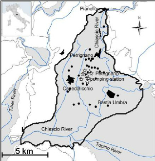
Petrignano Aquifer¶

Published studies on this topic:¶

On the variables to be considered in assessing the impact of climatechange to alluvial aquifers: a case study in central Italy. (2013), E. Romano, S. Camici, L. Brocca, T. Moramarco, F. Pica, E. Preziosi
The Sustainable Pumping Rate Concept: Lessons from a Case Study in Central Italy. (2009) Emanuele Romano, Elisabetta Preziosi, Italian National Research Council.

The-Petrignano-dAssisi-plain-Grey-areas-alluvial-deposits

In [5]:

petrignano=pd.read_csv(r"http://vanoproy.be/css/Aquifer_Petrignano.csv", sep=",", engine='python', encoding="UTF-8")# "
petrignano#.head(10) 

Out[5]:

	Date	Rainfall_Bastia_Umbra	Depth_to_Groundwater_P24	Depth_to_Groundwater_P25	Temperature_Bastia_Umbra	Temperature_Petrignano	Volume_C10_Petrignano	Hydrometry_Fiume_Chiascio_Petrignano
0	14/03/2006	NaN	-22.48	-22.18	NaN	NaN	NaN	NaN
1	15/03/2006	NaN	-22.38	-22.14	NaN	NaN	NaN	NaN
2	16/03/2006	NaN	-22.25	-22.04	NaN	NaN	NaN	NaN
3	17/03/2006	NaN	-22.38	-22.04	NaN	NaN	NaN	NaN
4	18/03/2006	NaN	-22.60	-22.04	NaN	NaN	NaN	NaN
...	...	...	...	...	...	...	...	...
5218	26/06/2020	0.0	-25.68	-25.07	25.7	24.5	-29930.688	2.5
5219	27/06/2020	0.0	-25.80	-25.11	26.2	25.0	-31332.960	2.4
5220	28/06/2020	0.0	-25.80	-25.19	26.9	25.7	-32120.928	2.4
5221	29/06/2020	0.0	-25.78	-25.18	26.9	26.0	-30602.880	2.4
5222	30/06/2020	0.0	-25.91	-25.25	27.3	26.5	-31878.144	2.4

5223 rows × 8 columns

In [6]:

petrignano["Date"] = pd.to_datetime( petrignano.Date, format='%d/%m/%Y' ) # euro dates
petrignano= petrignano.set_index("Date", inplace=False)

In [8]:

petrignano.head(6) 

Out[8]:

	Rainfall_Bastia_Umbra	Depth_to_Groundwater_P24	Depth_to_Groundwater_P25	Temperature_Bastia_Umbra	Temperature_Petrignano	Volume_C10_Petrignano	Hydrometry_Fiume_Chiascio_Petrignano
Date
2006-03-14	NaN	-22.48	-22.18	NaN	NaN	NaN	NaN
2006-03-15	NaN	-22.38	-22.14	NaN	NaN	NaN	NaN
2006-03-16	NaN	-22.25	-22.04	NaN	NaN	NaN	NaN
2006-03-17	NaN	-22.38	-22.04	NaN	NaN	NaN	NaN
2006-03-18	NaN	-22.60	-22.04	NaN	NaN	NaN	NaN
2006-03-19	NaN	-22.35	-21.95	NaN	NaN	NaN	NaN

In [ ]:

petrignano.info()

In [9]:

dfp =petrignano.rename(columns={'Rainfall_Bastia_Umbra':'Rain_Bastia','Depth_to_Groundwater_P24':'Depth_to_P24','Depth_to_Groundwater_P25':'Depth_to_P25', 
                   'Temperature_Bastia_Umbra':'Temp_Bastia', 'Temperature_Petrignano':'Temp_Petrig',"Volume_C10_Petrignano":"Volume_C10",
                   "Hydrometry_Fiume_Chiascio_Petrignano": "Hydrometry"})
dfp 

Out[9]:

	Rain_Bastia	Depth_to_P24	Depth_to_P25	Temp_Bastia	Temp_Petrig	Volume_C10	Hydrometry
Date
2006-03-14	NaN	-22.48	-22.18	NaN	NaN	NaN	NaN
2006-03-15	NaN	-22.38	-22.14	NaN	NaN	NaN	NaN
2006-03-16	NaN	-22.25	-22.04	NaN	NaN	NaN	NaN
2006-03-17	NaN	-22.38	-22.04	NaN	NaN	NaN	NaN
2006-03-18	NaN	-22.60	-22.04	NaN	NaN	NaN	NaN
...	...	...	...	...	...	...	...
2020-06-26	0.0	-25.68	-25.07	25.7	24.5	-29930.688	2.5
2020-06-27	0.0	-25.80	-25.11	26.2	25.0	-31332.960	2.4
2020-06-28	0.0	-25.80	-25.19	26.9	25.7	-32120.928	2.4
2020-06-29	0.0	-25.78	-25.18	26.9	26.0	-30602.880	2.4
2020-06-30	0.0	-25.91	-25.25	27.3	26.5	-31878.144	2.4

5223 rows × 7 columns

In [10]:

sns.set_style("whitegrid", {'grid.linestyle': '--'})
fig, ax = plt.subplots(4,1,  figsize=(21, 9), sharex=True) #, squeeze=False  

sns.lineplot(x="Date", y= petrignano["Rainfall_Bastia_Umbra"],data=petrignano, ax=ax[0])
sns.lineplot(x="Date", y= petrignano["Depth_to_Groundwater_P24"], data=petrignano, ax=ax[1]) # ax=ax
sns.lineplot(x="Date", y= petrignano["Depth_to_Groundwater_P25"], data=petrignano, ax=ax[2]) # ax=ax 
sns.lineplot(x="Date", y= petrignano["Hydrometry_Fiume_Chiascio_Petrignano"], data=petrignano, ax=ax[3]) # ax=ax 
plt.xticks(rotation=90); plt.grid(b=True,) #axe.setxaxis(rotation=90)
plt.xlim(pd.to_datetime( "2010-01-01" ),pd.to_datetime("2020-02-01" ) ); 

In [80]:

sns.set_style("whitegrid", {'grid.linestyle': '--'})
fig, ax = plt.subplots(4,1,  figsize=(21, 9), sharex=True) #, squeeze=False  

sns.lineplot(x="Date", y= petrignano["Rainfall_Bastia_Umbra"],data=petrignano, ax=ax[0])
sns.lineplot(x="Date", y= petrignano["Depth_to_Groundwater_P25"], data=petrignano, ax=ax[1]) # ax=ax
sns.lineplot(x="Date", y= petrignano["Temperature_Petrignano"], data=petrignano, ax=ax[2]) # ax=ax 
sns.lineplot(x="Date", y= petrignano["Hydrometry_Fiume_Chiascio_Petrignano"], data=petrignano, ax=ax[3]) # ax=ax 

plt.xticks(rotation=90); plt.grid(b=True,) #axe.setxaxis(rotation=90)
plt.xlim(pd.to_datetime( "2012-01-01" ),pd.to_datetime("2015-02-01" ) ); 

In [81]:

sns.set_style("whitegrid", {'grid.linestyle': '--'})
fig, ax = plt.subplots(4,1, figsize=(21, 9), sharex=True) #, squeeze=False  

sns.lineplot(x="Date", y= petrignano["Rainfall_Bastia_Umbra"],data=petrignano, ax=ax[0])
sns.lineplot(x="Date", y= petrignano["Depth_to_Groundwater_P24"], data=petrignano, ax=ax[1]); plt.ylim(-30,-25) # ax=ax
sns.lineplot(x="Date", y= petrignano["Temperature_Petrignano"], data=petrignano, ax=ax[2]); plt.ylim(0,4)# ax=ax 
sns.lineplot(x="Date", y= petrignano["Hydrometry_Fiume_Chiascio_Petrignano"], data=petrignano, ax=ax[3]);plt.ylim(0,4) # ax=ax 

plt.xticks(rotation=90); plt.grid(b=True,) #axe.setxaxis(rotation=90)
plt.xlim(pd.to_datetime( "2018-11-01" ),pd.to_datetime("2019-04-01" ) ); 

In [12]:

sns.set_style("whitegrid", {'grid.linestyle': '--'})
fig, ax = plt.subplots(2,1,  figsize=(21, 9), sharex=True) #, squeeze=False  

sns.lineplot(x="Date", y= dfp["Depth_to_P24"],data=dfp, ax=ax[0])
sns.lineplot(x="Date", y= dfp["Depth_to_P25"],data=dfp, ax=ax[0],color="forestgreen") # ax=ax
sns.lineplot(x="Date", y= dfp["Volume_C10"], data=dfp, ax=ax[1] ,color="olivedrab") # ax=ax 

plt.xticks(rotation=90); plt.grid(b=True,) #
plt.xlim(pd.to_datetime( "2006-09-19" ),pd.to_datetime("2007-09-01" ) ); 

Data refurbishment¶

We'll interpolate the missing values in the height data, and turn negative pumped volumes positive:

In [11]:

dfp.Depth_to_P24 =dfp.Depth_to_P24.interpolate(method="linear", limit_direction='forward') 
dfp.Depth_to_P25 =dfp.Depth_to_P25.interpolate(method="linear", limit_direction='forward') 

In [12]:

dfp.Volume_C10= -dfp.Volume_C10

Convertion of the volume of pumped water, expressed in cubic meters (mc) per day, to m³/s.

In [13]:

dfp["Debiet"]= dfp.Volume_C10/(3600*24)

In [14]:

dfp.describe()

Out[14]:

	Rain_Bastia	Depth_to_P24	Depth_to_P25	Temp_Bastia	Temp_Petrig	Volume_C10	Hydrometry	Debiet
count	4199.000000	5223.000000	5223.000000	4199.000000	4199.000000	5025.000000	4199.000000	5025.000000
mean	1.556633	-26.279945	-25.696110	15.030293	13.739081	29043.296726	2.372517	0.336149
std	5.217923	3.314307	3.222391	7.794871	7.701369	4751.864371	0.589088	0.054998
min	0.000000	-34.470000	-33.710000	-3.700000	-4.200000	-0.000000	0.000000	-0.000000
25%	0.000000	-28.265000	-27.630000	8.800000	7.700000	26218.080000	2.100000	0.303450
50%	0.000000	-26.020000	-25.540000	14.700000	13.500000	28689.120000	2.400000	0.332050
75%	0.100000	-23.840000	-23.430000	21.400000	20.000000	31678.560000	2.700000	0.366650
max	67.300000	-19.660000	-19.100000	33.000000	31.100000	45544.896000	4.100000	0.527140

During the first years P25's level is initially higher during the pumping, so it must be further away from well than P24. But the average pump rate lowers around 2014-2015, so the aquifer can get the opportunity to recharge partially.

In [15]:

print("P24min",dfp.Depth_to_P24.min(),"P25min", dfp.Depth_to_P25.min(),"P24max", dfp.Depth_to_P24.max(),"P25max",dfp.Depth_to_P25.max(), 
      round(dfp.Depth_to_P24.max()-dfp.Depth_to_P24.min(),2),dfp.Depth_to_P25.max()-dfp.Depth_to_P25.min())

P24min -34.47 P25min -33.71 P24max -19.66 P25max -19.1 14.81 14.61

I suppose that the original base of the suction cone is higher than the max. height of the provided depths. Later I'll use other heights based on groundlevel altitude above sealevel.

In [16]:

dfp["Hth_to_P24"]= dfp.Depth_to_P24.max()-dfp.Depth_to_P24
dfp["Hth_to_P25"]= dfp.Depth_to_P25.max()-dfp.Depth_to_P25; 

In [21]:

dfp["Hth_to_P25"].plot(); 

Note that 'Hth' is the heigth of the suction cone at a well, above the estimated "original" water table base level. In the plot you can notice that the average diff. in relative height shifts to the other side after 2013.

In [17]:

depthdiff= dfp.Hth_to_P24 -dfp.Hth_to_P25; sns.lineplot(data=depthdiff ); 

Somewhere in a published study I read that in the center of the aquifer the thickness is about 80 meters. I also saw in a published study that there has been an piezometric level of 170 meters in the aquifer center anno 2004. The location has an altitude of 200 m above sealevel.

In [18]:

dfp["CHt_P24"]= 80+ dfp.Depth_to_P24  # cone height at p24
dfp["CHt_P25"]= 80 +dfp.Depth_to_P25; 

In [23]:

dfp["CHt_P25"].plot(); 

We converted the water table level another time to be able to use the Dupuit formula, and a sea level heigth.

In [19]:

dfpsl=pd.DataFrame()
dfpsl["head24"]= 200+dfp.Depth_to_P24 ; 
dfpsl["head25"]= 200+dfp.Depth_to_P25; 
dfpsl.plot( figsize=(19, 4)); 
dfp["head24"]= 200+dfp.Depth_to_P24 ; 
dfp["head25"]= 200+dfp.Depth_to_P25; 

This is an image or a cross section of a pumped unconfined aquifer.

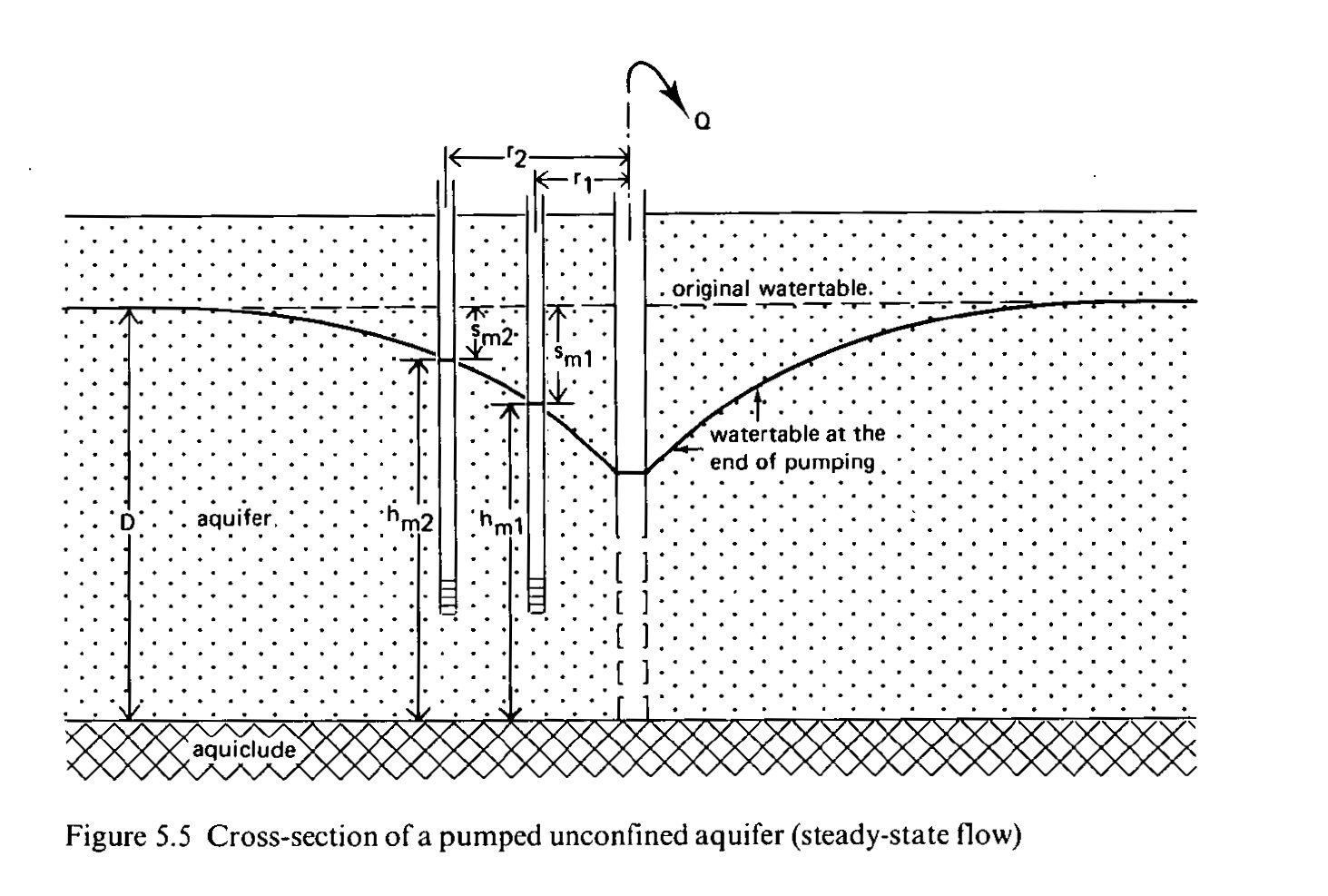
The next formula, based on the Dupuit formula, should result in a constant, but in this case it isn't, as there are fluctuations in the density of the soil. Also, there is competition from other pumping activities, and when they are excessive or nearby executed, they can lower the shape of the main well suction cone. The formula does not work near the well due to seepage.
In case the piezometer most far away from the well, P25, is located between P24 and the river, then water from the river can have positive or negative effects. But from the plots I deduct that the river water takes a month or more to arrive at the well site, so the effect on the slope is mild compared to others.

In [20]:

dfp["Hth2diff"]= (dfp.CHt_P25.rolling(7,min_periods=5).sum().fillna(method='bfill', limit=7) **2 -dfp.CHt_P24.rolling(7,min_periods=5).sum().fillna(method='bfill', limit=7)**2)/ (0.01+dfp.Volume_C10.rolling(7).sum().fillna(method='bfill', limit=7))
#dfp["Hth2diff"]= dfp["Hth2diff"].replace(np.nan,0) # why is this here, bit early
#dfp["Hth2diff"]= dfp.where( lambda x: dfp[dfp.Volume_C10==0], lambda x: 0)

In [21]:

dfp["Hth2diff_S1"]= (dfp.CHt_P25.rolling(7,min_periods=3).sum().fillna(method='bfill', limit=7).shift(1)**2 -dfp.CHt_P24.rolling(7,min_periods=3).sum().fillna(method='bfill', limit=7)**2)/(0.01+dfp.Volume_C10)
dfp["Hth2diff_S11"]= (dfp.CHt_P25.rolling(7,min_periods=3).sum().fillna(method='bfill', limit=7).shift(1)**2 -dfp.CHt_P24.rolling(7,min_periods=3).sum().fillna(method='bfill', limit=7).shift(1)**2)/(0.01+dfp.Volume_C10)
dfp["Hth2diff_S21"]= (dfp.CHt_P25.shift(2)**2 -dfp.CHt_P24.shift(1)**2)/(0.01+dfp.Volume_C10)

a plot with time shifts to get a better view on the fluctuations of the water levels.

In [72]:

sns.set_style("whitegrid", {'grid.linestyle': '--'}); fig, ax = plt.subplots(1,1, figsize=(23, 5), sharex=True)
#sns.lineplot(x=dfp.index, y=dfp["Hth2diff_S1"], data=dfp) ;# 
#sns.lineplot(x=dfp.index, y=dfp["Hth2diff_S11"], data=dfp ); #  2014-04-13    0.011207
#sns.lineplot(x=dfp.index, y=dfp["Hth2diff_S21"], data=dfp );  
sns.lineplot(x=dfp.index, y=dfp["Hth2diff"], data=dfp,ax=ax ); plt.ylim( .0,.03)
#sns.lineplot(x=dfp.index, y=dfp["Volume_C10"], data=dfp,ax=ax[1] ); plt.ylim( 15000,40000)
plt.xlim(pd.to_datetime( "2012-07-02" ),pd.to_datetime("2014-04-01" ) ); # "2010-04-01"

In [73]:

sns.set_style("whitegrid", {'grid.linestyle': '--'}); fig, ax = plt.subplots(1,1, figsize=(23, 5), sharex=True)
#sns.lineplot(x=dfp.index, y=dfp["Hth2diff_S1"], data=dfp) ;# 
#sns.lineplot(x=dfp.index, y=dfp["Hth2diff_S11"], data=dfp ); #  2014-04-13    0.011207
#sns.lineplot(x=dfp.index, y=dfp["Hth2diff_S21"], data=dfp );  
#sns.lineplot(x=dfp.index, y=dfp["Hth2diff"], data=dfp,ax=ax[0] ); plt.ylim( .0,.03)
sns.lineplot(x=dfp.index, y=dfp["Volume_C10"].rolling(90).sum() , data=dfp,ax=ax );
sns.lineplot(x=dfp.index, y=dfp["Volume_C10"], data=dfp,ax=ax ); plt.ylim( 20000,40000)

plt.xlim(pd.to_datetime( "2012-07-02" ),pd.to_datetime("2014-04-01" ) ); # "2010-04-01"

In [82]:

dfp["Hth2diff"]["2009-10-02":"2009-10-22"] 

Out[82]:

Date
2009-10-02    0.014837
2009-10-03    0.014863
2009-10-04    0.014794
2009-10-05    0.014341
2009-10-06    0.014232
2009-10-07    0.014128
2009-10-08    0.014168
2009-10-09    0.014004
2009-10-10    0.013911
2009-10-11    0.013761
2009-10-12    0.014191
2009-10-13    0.014145
2009-10-14    0.014043
2009-10-15    0.013934
2009-10-16    0.013846
2009-10-17    0.013673
2009-10-18    0.013800
2009-10-19    0.013541
2009-10-20    0.013652
2009-10-21    0.013670
2009-10-22    0.013503
Name: Hth2diff, dtype: float64

In [83]:

dfp["Hth2diff"].describe()

Out[83]:

count      5027.000000
mean         99.537152
std        4994.655440
min          -0.004075
25%           0.011687
50%           0.014767
75%           0.018150
max      262023.170000
Name: Hth2diff, dtype: float64

In [65]:

kwadrdf= dfp[["Volume_C10","Hth2diff_S11","Hth2diff_S21","Hth2diff_S1", "Hth2diff"]]
sns.heatmap( kwadrdf.corr(), annot=True ); 

In [66]:

sns.set_style("whitegrid", {'grid.linestyle': '--'})
fig, ax = plt.subplots(1,1, figsize=(19, 5), sharex=True);
sns.lineplot(data=dfp.head24, ax=ax) ;
sns.lineplot(data=dfp.head25, ax=ax); plt.ylim( 165,180); 
ax2= plt.twinx()
sns.lineplot( data=dfp.Volume_C10, ax=ax2,color="navy")
#plt.xlim(pd.to_datetime( "2006-05-01" ),pd.to_datetime("2010-07-01" ) );
plt.xlim(pd.to_datetime( "2008-11-30"),pd.to_datetime("2010-12-15" ) ); plt.ylim( 20000,45000);  

Dates which are lacking pumping data: 9/05/2007, 30/08/2007, 17/04/2008, 9/06/2011 and 10/06/2011, 20/12/2011; 12/07/2019 and 14/07/2019 No pumping periods: 2019-06-28: 2019-07-05], 2019-08-01: 2019-08-05]

In [23]:

import datetime
datetime.datetime(2006,9,25,0,0)

Out[23]:

datetime.datetime(2006, 9, 25, 0, 0)

Rainfall¶

In [74]:

print("Estimated drainage area of the aquifer:", 11.5*12.5/2, "km²")

Estimated drainage area of the aquifer: 71.875 km²

Conversion of rainfall units: mm/d to m³/d, for better comparison with pump abstraction values. Also the creation of an indicator for the month to be able to distinguish the months.

The actual drainage area for the source is not given, and here is an estimation based on info in a study of the geology of the alluvial plane.

In [22]:

pd.set_option('mode.chained_assignment',None)
dfp["Month"] =dfp.index.month

dfp["Rain_M³"] =dfp.Rain_Bastia* 72*1000.0*1000/ 1000 # 27km²
dfp["Rain_Log"] = np.log1p(dfp.Rain_Bastia) # Rain_M³

In [76]:

print("Estimated effective infiltration by the rain to aquifer:", round(250/(365*24*3600 ),8), "L/sec or ", round(250/365,2),"L/day")
effect_infil= 250/365* 72*1000.0; print( effect_infil, "m³")

Estimated effective infiltration by the rain to aquifer: 7.93e-06 L/sec or  0.68 L/day
49315.068493150684 m³

In [24]:

dfp["Rainfall_3"] =dfp.Rain_Bastia.rolling(3).sum().fillna(method='bfill', limit=3)
dfp["Rainfall_7"] =dfp.Rain_Bastia.rolling(7).sum().fillna(method='bfill', limit=7)
dfp["Rainfall_122"] =dfp.Rain_Bastia.rolling(122).sum().fillna(method='bfill', limit=122)
dfp["Rainfall_30"] =dfp.Rain_Bastia.rolling(30).sum().fillna(method='bfill', limit=30)

Temperature¶

We have obtained 2 temperature sets: Temp_Bastia and Temp_Petrig.

The temperature data for Petrignano in 2015 are flatlining from 2015-04-25 til 2015-09-21, 0's, and the weeks before that the device seems to be no longer correctly calibrated. What shall we do with such a series?
I'll also create a column to simulate a minimum temperature.

In [78]:

fig, ax = plt.subplots(1,1, figsize=(19, 6), sharex=True)
sns.lineplot(data=dfp.Temp_Bastia) ;
sns.lineplot(data=dfp.Temp_Petrig); 
plt.xlim(pd.to_datetime( "2014-02-01" ),pd.to_datetime("2015-05-01" ) ); plt.ylim(-0.5,30);

We perform a temperature correction for the Bastia data in the mentioned time period, in order to fill up the Petrignano data and use it.

In [25]:

dfp.Temp_Petrig["2015-04-25":"2015-09-21"] = dfp.Temp_Bastia["2015-04-25":"2015-09-21"]-0.75
dfp["TmnStdB"] =dfp.Temp_Bastia- dfp.Temp_Bastia.std(skipna=True)
dfp["TmnStdP"] =dfp.Temp_Petrig- dfp.Temp_Petrig.std(skipna=True)

Add some temperature rolling means that have a sort of minimum temp. behaviour.

In [26]:

dfp["TmnStdP_4"] =dfp.TmnStdP.rolling(4).mean().fillna(method='bfill', limit=3)
dfp["TP_7"] =dfp.Temp_Petrig.rolling(7).mean().fillna(method='bfill', limit=7)

On 2020-06-15 there is a nan in the pumped volume, which is the only exception. The aquifer might no longer be able to provide the amount of water...

In [27]:

sns.set_style("whitegrid", {'grid.linestyle': '--'})
fig, ax = plt.subplots(1,1, figsize=(19, 4.5), sharex=True);
sns.lineplot(data=dfp.head24, ax=ax) ;
sns.lineplot(data=dfp.head25, ax=ax); plt.ylim( 173,176); 
ax2= plt.twinx()
sns.lineplot( data=dfp.Volume_C10, ax=ax2,color="navy")
plt.xlim(pd.to_datetime( "2020-01-30"),pd.to_datetime("2020-06-30" ) ); plt.ylim( 15000,35000); 

fig, ax = plt.subplots(figsize=(17,5)) sns.lineplot(x= y_test.index,y= y_test.head24, data=y_test) #CHt_P25 Hth_to_P25 sns.lineplot(x= y_test.index,y= y_test.head25, data=y_test)

sns.lineplot(x= y_test.index,y= y_pred[:,0], data=y_pred) sns.lineplot(x= y_test.index,y= y_pred[:,1], data=y_pred);

Piezometer 24 has a nan at 2006-12-14, and from then on til 2007-04-28, it stays off indicating values about 25 cm higher. I'll subtract it

In [28]:

sns.set_style("whitegrid", {'grid.linestyle': '--'})
fig, ax = plt.subplots(1,1, figsize=(19, 5), sharex=True);
sns.lineplot(data=dfp.head24, ax=ax) ;
sns.lineplot(data=dfp.head25, ax=ax); plt.ylim( 165,180); 
ax2= plt.twinx()
sns.lineplot( data=dfp.Volume_C10, ax=ax2,color="navy")
plt.xlim(pd.to_datetime( "2008-11-30"),pd.to_datetime("2010-12-15" ) ); plt.ylim( 20000,45000);

No pumping¶

Dates which are lacking pumping data: 9/05/2007, 30/08/2007, 17/04/2008, 9/06/2011 and 10/06/2011, 20/12/2011; 12/07/2019 and 14/07/2019
No pumping periods: 2019-06-28: 2019-07-05], 2019-08-01: 2019-08-05]

Rainfall drainage area¶

In [30]:

print("Estimated drainage area of the aquifer:", 11.5*12.5/2, "km²", " study based area: 72-75 km²")

Estimated drainage area of the aquifer: 71.875 km²  study based area: 72-75 km²

Conversion of rainfall and discharge units: mm/d to m³/d, and creation of an indicator for the month to be able to distinguish the months or seasons.
The actual drainage area for the source is not given, and here is an estimation based on info in a study of the geology of the alluvial plane.

In [ ]:

pd.set_option('mode.chained_assignment',None)
dfp["Month"] =dfp.index.month

dfp["Rain_M³"] =dfp.Rain_Bastia* 721000.01000/ 1000 # 72km²
dfp["Rain_Log"] = np.log1p(dfp.Rain_Bastia) # Rain_M³

print("Estimated effective infiltration by the rain to aquifer:", round(250/(365243600 ),8), "L/sec or ", round(250/365,2),"L/day") dfp["Rainfall_3"] =dfp.Rain_Bastia.rolling(3).sum().fillna(method='bfill') dfp["Rainfall_7"] =dfp.Rain_Bastia.rolling(7).sum().fillna(method='bfill') dfp["Rainfall_122"] =dfp.Rain_Bastia.rolling(122).sum().fillna(method='bfill') dfp["Rainfall_30"] =dfp.Rain_Bastia.rolling(30).sum().fillna(method='bfill')

Discharge¶

Discharge, outtake, or pump volume, abstractions... are synonyms. There are some days when the volume is 0, which is caused by human intervention for reason of aquifer exhaustion, maintenance, safety inspection... These interruptions are exogenous in my opinion. I'm not sure what to do with them: drop, interpolate, ...

In [32]:

dfp.loc["Jun 2020"].Volume_C10= dfp.loc["Jun 2020"].Volume_C10.interpolate( limit_direction="forward")

In [33]:

dfp["Vol_124"]=dfp.Volume_C10.rolling(124).sum().fillna(method='bfill', limit=123) #
dfp["Vol_22"] =dfp.Volume_C10.rolling(22).sum().fillna(method='bfill', limit=22)
dfp["Vol_33"] =dfp.Volume_C10.rolling(30).sum().fillna(method='bfill', limit=30)
dfp["Vol_47"] =dfp.Volume_C10.rolling(47).sum().fillna(method='bfill', limit=47)

dfp.loc["2015-04-25":"2015-09-21"]

River Chiascio¶

river Chiascio The discharge average of the river is 20 m³/s. Let's find out the average of the water level over several years.

In [79]:

imC

Out[79]:

In [35]:

riverday= 20*3600*24; riveryr= 20*3600*24*365
print(f"Discharge average is {riverday:5,.0f} m³/d, {riveryr:5,.0f} m³/year")
dfp['doy'] = dfp.index.dayofyear
dfp['Year'] = dfp.index.year
dfp['Week'] = dfp.index.isocalendar().week

Discharge average is 1,728,000 m³/d, 630,720,000 m³/year

The river water level is 0 between 25/04/2015 and 21/09/2015. This could be a meteo station error or outfall. Shall I use nan?
No, I'll compute the average of river level for this period over several adjacent years.

In [36]:

piv = pd.pivot_table(dfp, index=['doy'],columns=['Year'], values=['Hydrometry'])
piv.plot( figsize=(19.8, 4));  # .groupby("Year")

I gonna make the average of timeseries data of adjacent years river level series to replace the missing data.

In [37]:

rivergap=pd.concat([dfp["2014-04-25":"2014-09-21"], dfp["2016-04-25":"2016-09-21"],dfp["2017-04-25":"2017-09-21"],dfp["2018-04-25":"2018-09-21"] ],ignore_index=True); rivergap

Out[37]:

	Rain_Bastia	Depth_to_P24	Depth_to_P25	Temp_Bastia	Temp_Petrig	Volume_C10	Hydrometry	Debiet	Hth_to_P24	Hth_to_P25	...	TmnStdP	TmnStdP_4	TP_7	Vol_124	Vol_22	Vol_33	Vol_47	doy	Year	Week
0	2.5	-20.09	-19.25	16.5	15.7	27427.680	2.8	0.31745	0.43	0.15	...	8.242949	8.442949	14.400000	3615595.488	607848.192	844175.520	1344589.632	115	2014	17
1	0.1	-19.99	-19.24	17.0	16.2	26551.584	2.8	0.30731	0.33	0.14	...	8.742949	8.242949	15.214286	3615242.112	606611.808	843095.520	1336940.640	116	2014	17
2	7.8	-19.71	-19.13	14.3	13.3	24432.192	2.7	0.28278	0.05	0.03	...	5.842949	7.542949	15.485714	3611040.480	602445.600	839655.072	1333412.928	117	2014	17
3	1.8	-19.80	-19.16	12.3	11.6	24573.024	2.7	0.28441	0.14	0.06	...	4.142949	6.742949	14.957143	3609717.696	598459.104	833086.080	1328408.640	118	2014	18
4	0.1	-19.91	-19.19	12.8	11.9	25180.416	2.7	0.29144	0.25	0.09	...	4.442949	5.792949	14.228571	3611186.496	595231.200	828808.416	1322829.792	119	2014	18
...	...	...	...	...	...	...	...	...	...	...	...	...	...	...	...	...	...	...	...	...	...
595	7.6	-25.74	-25.18	23.0	22.2	31367.520	2.3	0.36305	6.08	6.08	...	14.742949	15.992949	23.185714	3717809.280	682622.208	934350.336	1444591.584	260	2018	38
596	13.0	-25.78	-25.25	22.3	21.7	29403.648	2.4	0.34032	6.12	6.15	...	14.242949	15.542949	23.014286	3720457.440	683049.888	934301.952	1440867.744	261	2018	38
597	0.2	-25.90	-25.28	21.9	21.8	29782.944	2.3	0.34471	6.24	6.18	...	14.342949	15.092949	22.700000	3723190.272	683335.872	932164.416	1444997.664	262	2018	38
598	0.0	-25.65	-25.20	22.5	22.5	27522.720	2.3	0.31855	5.99	6.10	...	15.042949	14.592949	22.828571	3722259.744	680270.400	926876.736	1438293.024	263	2018	38
599	0.0	-25.70	-25.19	23.3	23.2	30092.256	2.2	0.34829	6.04	6.09	...	15.742949	14.842949	22.785714	3725691.552	678843.936	924373.728	1438006.176	264	2018	38

600 rows × 34 columns

In [39]:

riverHydro=rivergap.loc[:,["Hydrometry","doy"]]; 

In [40]:

riverHydroavg=riverHydro.groupby("doy").mean() #  .Hydrometry  axis=1
riverHydro.groupby("doy").mean().plot(); 

In [ ]:

dfp.groupby("doy")["Hydrometry"].mean().plot(); 

and we update the original with the averages of the adjacent years for the period which has missing data.

In [41]:

riverHydroavg= riverHydroavg[:-1]
riverHydroavg.index = dfp["2015-04-25":"2015-09-21"].index
dfp.update(riverHydroavg)

Collected information and considerations¶

This is information that I retrieved from publicated studies. I also added my own considerations.

I wanna make an indicator or weighted factor, based on the timely water budget of aquifer state and water level of the stream.
How far is the river away from the measure pits?
- About 1900 meters, which means this river water can take a while to flow through the soil to the suction coil.
Can I find out which measure pits is closest to the stream Chiascio?
- P25 had the heighest level during the intensive pumping times.
The influence of the river level on the difference in cone height vs. the relative head of the closest measurement.

Some author wrote that the aquifer hasn't been in a steady-state since 2001.
The possible recharge of the aquifer, and the difference between surface water and groundwater levels, are influenced by pumping rate. But, there is also well pumping by agricultural and private actors happening, esp. when it's warm and dry (during May-September).
This is a dynamic system, which consists of 4 drivers: recharge by rain, aquifer storage, pump outtake and drain to river. The latter can be positive or negative. The variation in recharge influences the aquifer storage and the drain to river, and the variation in abstraction influences storage and drain to river. These variations have different time lags.
On top of that there are 2 scenario's: the northern part of the river can feed the aquifer, while the southern part of the stream role depends on the balance btn. groundwater level and the amount of abstractions.

In [ ]:

imGWI

dfp["diff_surface_gwater"] =((dfp.Hydrometry.rolling(128).mean(min_periods=1))*(dfp.head25**2-dfp.head24**2))/ -(dfp.head24/(0.00000000001+dfp.head24.max()-dfp.head24.min()))#**2 #.rolling(3).sum()

dfp["2009":"2020"]["diff_surface_gwater"].plot(); # -np.log1p( .fillna('bfill')

sns.set_style("whitegrid", {'grid.linestyle': '--'}) fig, ax = plt.subplots(1,1, figsize=(19, 4.5), sharex=True); sns.lineplot(data=dfp.Rain_Bastia.rolling(3).mean(), ax=ax) ; sns.lineplot(data=dfp.diff_surface_gwater.rolling(3).mean(), ax=ax); #plt.ylim( 0,8); ax2= plt.twinx() sns.lineplot( data=dfp.Volume_C10.rolling(3).mean(), ax=ax2,color="navy"); plt.ylim( 20000,35000); plt.xlim(pd.to_datetime( "2010-01-30"),pd.to_datetime("2010-12-30" ) );

In [42]:

dfp["Hyd_39"] =dfp.Hydrometry.rolling(39).sum().fillna(method='bfill', limit=39)  # level to m³ ?  or
dfp["Hyd_128"] =dfp.Hydrometry.rolling(128).sum().fillna(method='bfill', limit=128) 
#dfp["HydStd_8"]=dfp.Hydrometry.rolling(8).std().fillna(method='bfill') 
dfp["2009":"2020"].Hydrometry.plot( lw=0.5);   # level to m³ ?

Minimum and max. ground water levels over the years¶

From 2008 to 2012 there has been a period of exhaustion of the aquifer storage, which led to more and more lower headings for the water levels. Since 2013-2014 the pumping rate has been somewhat reduced in order to give the aquifer time to replenish.

In [43]:

dfp['Year'] = dfp.index.year
Min_year = dfp["2008-01-01":"2020-04-01"].groupby('Year')[["Hth_to_P24","Hth_to_P25"]].min(); 
MinVol_year = dfp["2008-01-01":"2020-04-01"].groupby('Year')[["Volume_C10"]].mean(); 
Max_year = dfp["2008-01-01":"2020-04-01"].groupby('Year')[["Hth_to_P24","Hth_to_P25"]].min();
MaxVol_year = dfp["2008-01-01":"2020-04-01"].groupby('Year')[["Volume_C10"]].max();

In [44]:

sns.set_style("whitegrid", {'grid.linestyle': '--'})
fig, ax = plt.subplots(2,1,  figsize=(10.7, 6), sharex=True) #  
plt.grid()
sns.lineplot(data=Min_year, label="Min height  year",ax=ax[0] )# x=Rain_Bastia_month.index, y= "Rain_Bastia", 
sns.lineplot(data=Max_year, label="Max height  year",ax=ax[0] )
#ax[0].axis(xmin=0 ,xmax=15 ) # xlim( 0,)          x=Volume_C10_month.index, y= "Volume_C10", 
sns.lineplot(data=MinVol_year, label="Avg vol  year",color="coral", ax=ax[1]) # ax=ax
sns.lineplot(data=MaxVol_year, label="Max vol",color="coral", ax=ax[1]) 
#sns.lineplot(x=dfp.index, y= "RainNO_2", data=dfp, label="Rain NE", ax=ax[2]) # 
plt.xticks(rotation=90); 
#plt.xlim(pd.to_datetime( "2010-01-01" ),pd.to_datetime("2019-12-31" ) ); 

Monthly rainfall and pump volume¶

In [45]:

Rain_Bastia_month = dfp["2009-01-01":"2020-04-01"].groupby('Month')[["Rain_Bastia"]].sum(); 
Volume_C10_month = dfp["2009-01-01":"2020-04-01"].groupby('Month')[["Volume_C10"]].mean(); 
Volume_sum_month = dfp["2009-01-01":"2020-04-01"].groupby('Month')[["Volume_C10"]].sum(); 
Hydro_month = dfp["2009-01-01":"2020-04-01"].groupby('Month')[["Hydrometry"]].sum(); 
Volume_C10_month 

Out[45]:

	Volume_C10
Month
1	28521.204387
2	28203.098336
3	27683.219613
4	27834.916350
5	27676.240891
6	28236.006982
7	29313.153501
8	29050.016094
9	29954.149527
10	30072.384000
11	29789.395200
12	28688.220528

In [46]:

sns.set_style("whitegrid", {'grid.linestyle': '--'})
fig, ax = plt.subplots(2,1,  figsize=(17, 5), sharex=True) #  plt.grid()
sns.lineplot(x=Rain_Bastia_month.index, y= "Rain_Bastia", data=Rain_Bastia_month, label="Rain_Bastia_month",ax=ax[0] )
#ax[0].axis(xmin=0 ,xmax=15 ) # xlim( 0,)
sns.lineplot(x=Volume_C10_month.index, y= "Volume_C10", data=Volume_C10_month, label="Volume_C10_month",color="coral", ax=ax[1]) # ax=ax
#sns.lineplot(x=dfp.index, y= "RainNO_2", data=dfp, label="Rain NE", ax=ax[2]) # 
plt.xticks(rotation=90); #axe.setxaxis(rotation=90)
#plt.xlim(pd.to_datetime( "2010-01-01" ),pd.to_datetime("2019-12-31" ) ); 

Autocorrelation¶

The change in pump regime is visible in this period: notice the dips: 8, 25, and peaks: 14, 33, 47.

In [47]:

import statsmodels.api as sm #figsize=(10, 3)
sm.graphics.tsa.plot_acf(dfp["2018-01-01":"2020-04-01"].Volume_C10.values, lags=80, color='indigo',markersize=3) #.squeeze()
plt.show()

In [48]:

import statsmodels.api as sm #figsize=(10, 3)
sm.graphics.tsa.plot_acf(dfp["2015-01-01":"2020-04-01"].Volume_C10.values, lags=80, color='indigo',markersize=3) #.squeeze()
plt.show()

In [49]:

import statsmodels.api as sm
sm.graphics.tsa.plot_acf(dfp["2010-04-01":"2015-04-01"].Volume_C10.values, lags=80, color='indigo',markersize=3) #.squeeze()
plt.show()

In [50]:

import statsmodels.api as sm
sm.graphics.tsa.plot_acf(dfp["2010-04-01":"2020-04-01"].Volume_C10.values, lags=80, color='indigo',markersize=3) #.squeeze()
plt.show()

In [51]:

import statsmodels.api as sm
sm.graphics.tsa.plot_acf(dfp["2010-04-01":"2020-04-01"].Hydrometry.values, lags=360, color='indigo',markersize=3) #.squeeze()
plt.show()

In [52]:

import statsmodels.api as sm
sm.graphics.tsa.plot_acf(dfp["2010-01-01":"2020-04-01"].head25.values, lags=80, color='indigo',markersize=3) #.squeeze()
plt.show()

In [53]:

import statsmodels.api as sm
sm.graphics.tsa.plot_acf(dfp["2010-01-01":"2020-04-01"].Rain_Bastia.values, lags=360, color='indigo',markersize=3) #.squeeze()
plt.show()

Seasonal decompose¶

In [54]:

from sklearn.feature_selection import RFE
from sklearn.ensemble import ExtraTreesRegressor

In [ ]:

from statsmodels.tsa.seasonal import seasonal_decompose
dfpseason = dfp[['Rain_Bastia', 'Depth_to_P24', 'Depth_to_P25', 
       'Temp_Petrig', 'Volume_C10', 'Hydrometry',       'head24', 'head25', 'Hth2diff',
       'Month', 'Rainfall_3', 'Rainfall_7', 'Rainfall_122', 'Rainfall_30',
      'TmnStdP', 'TmnStdP_4', 'TP_7', 'Vol_124', 'Vol_22',
       'Vol_33', 'Vol_47', 'doy', 'Year', 'Hyd_39', 'Hyd_128']] #  'diff_surface_gwater',

dfpseason['head25nextday'] = dfpseason['head25'].shift(-1)
dfpseason = dfpseason.dropna()
dfpseason = dfpseason.reset_index()
decompose_columns =  ['Rain_Bastia', 'Temp_Petrig', 'head25','Volume_C10',"Hydrometry"]

for column in decompose_columns:
    decompose_data = seasonal_decompose(dfpseason[column], freq=52, model='additive', extrapolate_trend='freq')# period n days! not weeks 
    dfpseason[f"{column}_Trend"] = decompose_data.trend
    dfpseason[f"{column}_Seasonal"] = decompose_data.seasonal

f, ax = plt.subplots(nrows=12, ncols=1, figsize=(19, 20))
f.tight_layout()
f.subplots_adjust(hspace=0.5)

sns.lineplot(x=dfpseason.Date, y=dfpseason.Rain_Bastia, data=dfpseason, ax=ax[0], color='black')
ax[0].set_title('Rainfall', fontsize=10)
ax[0].set_ylabel(ylabel=' ')
ax[0].set_xlabel(xlabel=' ')
sns.lineplot(x=dfpseason.Date, y=dfpseason.Rain_Bastia_Trend, ax=ax[1], color='black')
ax[1].set_title('Rainfall_Trend', fontsize=10)
ax[1].set_ylabel(ylabel=' ')
ax[1].set_xlabel(xlabel=' ');

sns.lineplot(x=dfpseason.Date, y=dfpseason.Rain_Bastia_Seasonal, data=dfpseason, ax=ax[2], color='black')
ax[2].set_title('Rainfall_Seasonal', fontsize=10)
ax[2].set_ylabel(ylabel=' ')
ax[2].set_xlabel(xlabel=' ')
sns.lineplot(x=dfpseason.Date, y=dfpseason.Temp_Petrig, ax=ax[3], color='black')
ax[3].set_title('Temperature_Petrig', fontsize=10)
ax[3].set_ylabel(ylabel=' ')
ax[3].set_xlabel(xlabel=' ')
sns.lineplot(x=dfpseason.Date, y=dfpseason.Temp_Petrig_Trend, ax=ax[4], color='black')
ax[4].set_title('Temperature_Petrig_Trend', fontsize=10)
ax[4].set_ylabel(ylabel=' ')
ax[4].set_xlabel(xlabel=' ')
sns.lineplot(x=dfpseason.Date, y=dfpseason.Temp_Petrig_Seasonal, ax=ax[5], color='black')
ax[5].set_title('Temperature_Petrig_Seasonal', fontsize=10)
ax[5].set_ylabel(ylabel=' ')
ax[5].set_xlabel(xlabel=' ')
sns.lineplot(x=dfpseason.Date, y=dfpseason.Hydrometry, ax=ax[6], color='black')
ax[6].set_title('Hydrometry', fontsize=10)
ax[6].set_ylabel(ylabel=' ')
ax[6].set_xlabel(xlabel=' ')
sns.lineplot(x=dfpseason.Date, y=dfpseason.Hydrometry_Trend, ax=ax[7], color='black')
ax[7].set_title('Hydrometry_Trend', fontsize=10)
ax[7].set_ylabel(ylabel=' ')
ax[7].set_xlabel(xlabel=' ')
sns.lineplot(x=dfpseason.Date, y=dfpseason.Hydrometry_Seasonal, ax=ax[8], color='black')
ax[8].set_title('Hydrometry_Season', fontsize=10)
ax[8].set_ylabel(ylabel=' ')
ax[8].set_xlabel(xlabel=' ')
sns.lineplot(x=dfpseason.Date, y=dfpseason.Volume_C10, ax=ax[9], color='black')
ax[6].set_title('Volume_C10', fontsize=10)
ax[6].set_ylabel(ylabel=' ')
ax[6].set_xlabel(xlabel=' ')
sns.lineplot(x=dfpseason.Date, y=dfpseason.Volume_C10_Trend, ax=ax[10], color='black')
ax[7].set_title('Volume_C10y_Trend', fontsize=10)
ax[7].set_ylabel(ylabel=' ')
ax[7].set_xlabel(xlabel=' ')
sns.lineplot(x=dfpseason.Date, y=dfpseason.Volume_C10_Seasonal, ax=ax[11], color='black')
ax[8].set_title('Volume_C10_Season', fontsize=10)
ax[8].set_ylabel(ylabel=' ')
ax[8].set_xlabel(xlabel=' ')
plt.show()

period of 180 days¶

In [55]:

from statsmodels.tsa.seasonal import seasonal_decompose

dfpseason = dfp[['Rain_Bastia', 'Depth_to_P24', 'Depth_to_P25', 
       'Temp_Petrig', 'Volume_C10', 'Hydrometry',       'head24', 'head25', 'Hth2diff',
       'Month', 'Rainfall_3', 'Rainfall_7', 'Rainfall_122', 'Rainfall_30',
      'TmnStdP', 'TmnStdP_4', 'TP_7', 'Vol_124', 'Vol_22',
       'Vol_33', 'Vol_47', 'doy', 'Year', 'Hyd_39', 'Hyd_128']] #'diff_surface_gwater',

dfpseason['head25nextday'] = dfpseason['head25'].shift(-1)
dfpseason = dfpseason.dropna()
dfpseason = dfpseason.reset_index()
decompose_columns =  ['Rain_Bastia', 'Temp_Petrig', 'head25','Volume_C10',"Hydrometry"]

for column in decompose_columns:
    decompose_data = seasonal_decompose(dfpseason[column], period=180, model='additive', extrapolate_trend='freq')# period n days! not weeks 
    dfpseason[f"{column}_Trend"] = decompose_data.trend
    dfpseason[f"{column}_Seasonal"] = decompose_data.seasonal

f, ax = plt.subplots(nrows=12, ncols=1, figsize=(19, 20))
f.tight_layout()
f.subplots_adjust(hspace=0.5)
sns.lineplot(x=dfpseason.Date, y=dfpseason.Rain_Bastia, data=dfpseason, ax=ax[0], color='black')
ax[0].set_title('Rainfall', fontsize=10)
ax[0].set_ylabel(ylabel=' ')
ax[0].set_xlabel(xlabel=' ')

sns.lineplot(x=dfpseason.Date, y=dfpseason.Rain_Bastia_Trend, ax=ax[1], color='black')
ax[1].set_title('Rainfall_Trend', fontsize=10)
ax[1].set_ylabel(ylabel=' ')
ax[1].set_xlabel(xlabel=' ');

sns.lineplot(x=dfpseason.Date, y=dfpseason.Rain_Bastia_Seasonal, data=dfpseason, ax=ax[2], color='black')
ax[2].set_title('Rainfall_Seasonal', fontsize=10)
ax[2].set_ylabel(ylabel=' ')
ax[2].set_xlabel(xlabel=' ')
sns.lineplot(x=dfpseason.Date, y=dfpseason.head25, ax=ax[3], color='black')
ax[3].set_title('head25', fontsize=10)
ax[3].set_ylabel(ylabel=' ')
ax[3].set_xlabel(xlabel=' ')
sns.lineplot(x=dfpseason.Date, y=dfpseason.head25_Trend, ax=ax[4], color='black')
ax[4].set_title('head25_Trend', fontsize=10)
ax[4].set_ylabel(ylabel=' ')
ax[4].set_xlabel(xlabel=' ')
sns.lineplot(x=dfpseason.Date, y=dfpseason.head25_Seasonal, ax=ax[5], color='black')
ax[5].set_title('head25_Seasonal', fontsize=10)
ax[5].set_ylabel(ylabel=' ')
ax[5].set_xlabel(xlabel=' ')
sns.lineplot(x=dfpseason.Date, y=dfpseason.Hydrometry, ax=ax[6], color='black')
ax[6].set_title('Hydrometry', fontsize=10)
ax[6].set_ylabel(ylabel=' ')
ax[6].set_xlabel(xlabel=' ')
sns.lineplot(x=dfpseason.Date, y=dfpseason.Hydrometry_Trend, ax=ax[7], color='black')
ax[7].set_title('Hydrometry_Trend', fontsize=10)
ax[7].set_ylabel(ylabel=' ')
ax[7].set_xlabel(xlabel=' ')
sns.lineplot(x=dfpseason.Date, y=dfpseason.Hydrometry_Seasonal, ax=ax[8], color='black')
ax[8].set_title('Hydrometry_Seasonal', fontsize=10)
ax[8].set_ylabel(ylabel=' ')
ax[8].set_xlabel(xlabel=' ')
sns.lineplot(x=dfpseason.Date, y=dfpseason.Volume_C10, ax=ax[9], color='black')
ax[6].set_title('Volume_C10', fontsize=10)
ax[6].set_ylabel(ylabel=' ')
ax[6].set_xlabel(xlabel=' ')
sns.lineplot(x=dfpseason.Date, y=dfpseason.Volume_C10_Trend, ax=ax[10], color='black')
ax[7].set_title('Volume_C10y_Trend', fontsize=10)
ax[7].set_ylabel(ylabel=' ')
ax[7].set_xlabel(xlabel=' ')
sns.lineplot(x=dfpseason.Date, y=dfpseason.Volume_C10_Seasonal, ax=ax[11], color='black')
ax[8].set_title('Volume_C10_Seasonal', fontsize=10)
ax[8].set_ylabel(ylabel=' ')
ax[8].set_xlabel(xlabel=' ')
plt.show()

<ipython-input-55-a263334b80b4>:15: FutureWarning: the 'freq'' keyword is deprecated, use 'period' instead
  decompose_data = seasonal_decompose(dfpseason[column], freq=180, model='additive', extrapolate_trend='freq')# period n days! not weeks

In [ ]:

Hydrological models¶

Pastas seems a nice framework for hydrological models, but it is necessary to use the correct unit for certain features. Also finding some usefull evaporation data for Italy was an obstacle.

!pip install pastas

In [56]:

import pastas as ps

###### Import groundwater time series and squeeze to Series object
gwdata = dfp.head25  #pd.read_csv('Aquifer_Petrignano.csv', parse_dates=['date'], index_col='date', squeeze=True)
print('The data type of the oseries is: %s' % type(gwdata))

###### Plot the observed groundwater levels
gwdata.plot(style='.', figsize=(17, 4), markersize=2.4)
plt.ylabel('Head [m]');
plt.xlabel('Time [years]');

The data type of the oseries is: <class 'pandas.core.series.Series'>

In [ ]:

# Import observed precipitation series
#precip = dfp.Rain_Bastia #Rain_Prepignano  #pd.read_csv('../data/rain_nb1.csv', parse_dates=['date'], index_col='date', squeeze=True)
#print('The data type of the precip series is: %s' % type(precip))

# Import observed evaporation series
#evap = pd.read_csv(r'../input/nb18_evap.csv', parse_dates=['date'], index_col='date', squeeze=True)
#evap = evap.loc["2008":"2021"]
#print('The data type of the evap series is: %s' % type(evap))

# Calculate the recharge to the groundwater
#recharge = precip - evap

# Plot the time series of the precipitation and evaporation
#plt.figure()
#recharge.plot(label='Recharge', figsize=(17, 4))
#plt.xlabel('Time [years]')
#plt.ylabel('Recharge (m/year)');

Create a time series model¶

In this code block the actual time series model is created. First, an instance of the Model class is created (named ml here). Second, the different components of the time series model are created and added to the model. The imported time series are automatically checked for missing values and other inconsistencies. The keyword argument fillnan can be used to determine how missing values are handled. If any nan-values are found this will be reported by pastas.

Here we remove most of the 0's from the volume series. Perhaps it is better to remove them all.

In [57]:

from pandas import Timestamp
strikedaystodump =[Timestamp('2011-06-10 00:00:00'), Timestamp('2019-06-29 00:00:00'),
 Timestamp('2019-06-30 00:00:00'), Timestamp('2019-07-01 00:00:00'),
 Timestamp('2019-07-02 00:00:00'), #Timestamp('2019-07-03 00:00:00'),
 Timestamp('2019-07-04 00:00:00'), Timestamp('2019-07-05 00:00:00'),
 Timestamp('2019-07-14 00:00:00'), Timestamp('2019-07-21 00:00:00'),
 Timestamp('2019-08-01 00:00:00'), Timestamp('2019-08-05 00:00:00'),
 Timestamp('2019-08-14 00:00:00'), Timestamp('2019-08-16 00:00:00'),
 Timestamp('2019-08-19 00:00:00'), Timestamp('2019-08-21 00:00:00')]
dfp=dfp[ ~dfp.index.isin(strikedaystodump)]

In [ ]:

Single target regression for Petrignano¶

First I'll try the RandomForestRegressor, to predict 1 of the 2 headings/cone heights based on the pure - or some transformation(s)- of the other heading/cone height.
I should find a factor which brings in the weight of rainfall (and evaporation), river level and pump discharge, based on the waterbalance...
after that ... Keras or XGBoost.

There are some days when the volume is 0, which is caused by human intervention I believe. These records are unpure, and distort the series, so I'll only keep the first day, and the rest will be dropped.

In [58]:

# Just take dates with decent data...train the model, and predict the 2020 values
dfp08= dfp["2009-01-01":"2020-06-14"]
dfp08.replace([np.inf, -np.inf], np.nan, inplace=True)
dfp08= dfp08.dropna() # inplace=True

Depth_to_P24= dfp08.loc[:,["head25"]]# "CHt_P25"
Petri= dfp08.drop(columns= ["Hth_to_P24","Hth_to_P25","Depth_to_P24","Depth_to_P25","CHt_P24","CHt_P25","head24","head25"], axis=1)
Petri.head()   # ,"depthdiff","depth2diff","Hthdiff", "Hth2diff","T_Delta"        #

Out[58]:

	Rain_Bastia	Temp_Bastia	Temp_Petrig	Volume_C10	Hydrometry	Debiet	Hth2diff	Hth2diff_S1	Hth2diff_S11	Hth2diff_S21	...	TP_7	Vol_124	Vol_22	Vol_33	Vol_47	doy	Year	Week	Hyd_39	Hyd_128
Date
2009-01-01	0.0	5.2	4.9	24530.688	2.4	0.28392	0.021735	0.153637	0.167255	0.003378	...	1.285714	4085576.064	626293.728	861848.640	1404765.504	1	2009	1	94.9	312.5
2009-01-02	0.0	2.3	2.5	28785.888	2.5	0.33317	0.021625	0.135752	0.141561	0.002117	...	1.285714	4080887.136	627008.256	861249.888	1402965.792	2	2009	1	94.9	312.5
2009-01-03	0.0	4.4	3.9	25766.208	2.4	0.29822	0.021607	0.148980	0.162234	0.003345	...	1.285714	4070869.920	621679.104	857704.032	1395009.216	3	2009	1	94.9	312.5
2009-01-04	0.0	0.8	0.8	27919.296	2.4	0.32314	0.021496	0.140069	0.147994	0.002985	...	1.285714	4063772.160	613121.184	857570.976	1392793.056	4	2009	1	94.9	312.5
2009-01-05	0.0	-1.9	-2.1	29854.656	2.3	0.34554	0.021474	0.132703	0.139222	0.002730	...	1.285714	4057692.192	610816.032	855811.872	1391827.968	5	2009	2	94.9	312.5

5 rows × 28 columns

In [59]:

print(Petri.shape, Depth_to_P24.shape )

(4168, 28) (4168, 1)

In [60]:

Petri.iloc[:,0:15].head(10)

Out[60]:

	Rain_Bastia	Temp_Bastia	Temp_Petrig	Volume_C10	Hydrometry	Debiet	Hth2diff	Hth2diff_S1	Hth2diff_S11	Hth2diff_S21	Month	Rainfall_3	Rainfall_7	Rainfall_122	Rainfall_30
Date
2009-01-01	0.0	5.2	4.9	24530.688	2.4	0.28392	0.021735	0.153637	0.167255	0.003378	1	0.0	0.0	70.8	6.3
2009-01-02	0.0	2.3	2.5	28785.888	2.5	0.33317	0.021625	0.135752	0.141561	0.002117	1	0.0	0.0	70.8	6.3
2009-01-03	0.0	4.4	3.9	25766.208	2.4	0.29822	0.021607	0.148980	0.162234	0.003345	1	0.0	0.0	70.8	6.3
2009-01-04	0.0	0.8	0.8	27919.296	2.4	0.32314	0.021496	0.140069	0.147994	0.002985	1	0.0	0.0	70.8	6.3
2009-01-05	0.0	-1.9	-2.1	29854.656	2.3	0.34554	0.021474	0.132703	0.139222	0.002730	1	0.0	0.0	70.8	6.3
2009-01-06	0.0	-0.7	-0.7	29124.576	2.3	0.33709	0.021617	0.136174	0.144477	0.002964	1	0.0	0.0	70.8	6.3
2009-01-07	0.0	1.5	-0.3	31173.120	2.3	0.36080	0.021595	0.128451	0.135785	0.002741	1	0.0	0.0	70.8	6.3
2009-01-08	0.0	4.3	6.6	30232.224	2.4	0.34991	0.021233	0.137938	0.140831	0.002922	1	0.0	0.0	70.8	6.3
2009-01-09	0.9	4.9	4.8	30597.696	2.3	0.35414	0.020892	0.135710	0.140771	0.002764	1	0.9	0.9	70.8	6.3
2009-01-10	0.0	1.9	4.2	31337.280	2.3	0.36270	0.020318	0.131932	0.136447	0.002669	1	0.9	0.9	70.8	6.3

we drop some features that proved not to progress the model after several train and test runs. at random several combinations were used.

In [61]:

Petri= Petri.drop(columns=["Temp_Bastia","TmnStdB",'Rain_Bastia','Temp_Petrig','Volume_C10','Hth2diff_S1','Hth2diff_S11','Hth2diff_S21',#'Rainfall_3','Rainfall_30',  'Volume_C10', 
                           'TmnStdP', "TmnStdP_4",'Hydrometry','Debiet','Rainfall_3','Rainfall_7',"Rainfall_30", 'TmnStdP'], axis=1) #,'HydStd_8' "Hthdiff","Year",   ,'Hth2diff'

In [62]:

X= Petri
y= Depth_to_P24
print(X.shape,y.shape )

(4168, 14) (4168, 1)

In [63]:

from sklearn.metrics import mean_squared_error
from sklearn.model_selection import train_test_split
from sklearn.model_selection import TimeSeriesSplit 
from sklearn.ensemble import RandomForestRegressor
#from sklearn.ensemble import ExtraTreesRegressor
from sklearn.feature_selection import SelectFromModel
from sklearn.metrics import accuracy_score

X_train,X_test, y_train,y_test= train_test_split(X ,y, test_size=0.105,random_state=1108,shuffle=False,)# ,n_splits=9.0max_train_size=365 random_state=1100,shuffle=Fals

X_train = X_train.values.reshape(-1,1) X_test = X_test.values.reshape(-1,1)

In [64]:

print(X_train.shape, y_train.shape, X_test.shape,y_test.shape)

(3730, 14) (3730, 1) (438, 14) (438, 1)

col_mask= X_train.isnull().any(axis=0); row_mask= X_train.isnull().any(axis=1); X_train.loc[row_mask,col_mask]

from Random Forest Regressor to Extra Trees Regressor¶

In [65]:

from sklearn.ensemble import GradientBoostingRegressor
from sklearn.ensemble import RandomForestRegressor
from sklearn.ensemble import ExtraTreesRegressor
#from sklearn.linear_model import LinearRegression
from sklearn.model_selection import cross_val_score
from sklearn import preprocessing
from sklearn.preprocessing import StandardScaler

sc = StandardScaler()
X_train = sc.fit_transform(X_train)
X_test = sc.transform(X_test)

#GBr = GradientBoostingRegressor(random_state=100)
RFr = ExtraTreesRegressor(random_state=1100, n_jobs=3, n_estimators=12300,bootstrap=True,verbose=1,criterion="mse",max_features=None,min_samples_leaf=1)# log

In [ ]:

type(X_train)

In [66]:

RFr.fit(X_train, y_train.values.ravel()) 

[Parallel(n_jobs=3)]: Using backend ThreadingBackend with 3 concurrent workers.
[Parallel(n_jobs=3)]: Done  44 tasks      | elapsed:    0.0s
[Parallel(n_jobs=3)]: Done 194 tasks      | elapsed:    0.5s
[Parallel(n_jobs=3)]: Done 444 tasks      | elapsed:    1.1s
[Parallel(n_jobs=3)]: Done 794 tasks      | elapsed:    2.1s
[Parallel(n_jobs=3)]: Done 1244 tasks      | elapsed:    3.4s
[Parallel(n_jobs=3)]: Done 1794 tasks      | elapsed:    5.1s
[Parallel(n_jobs=3)]: Done 2444 tasks      | elapsed:    7.1s
[Parallel(n_jobs=3)]: Done 3194 tasks      | elapsed:    9.7s
[Parallel(n_jobs=3)]: Done 4044 tasks      | elapsed:   12.8s
[Parallel(n_jobs=3)]: Done 4994 tasks      | elapsed:   16.3s
[Parallel(n_jobs=3)]: Done 6044 tasks      | elapsed:   21.1s
[Parallel(n_jobs=3)]: Done 7194 tasks      | elapsed:   27.1s
[Parallel(n_jobs=3)]: Done 8444 tasks      | elapsed:   33.8s
[Parallel(n_jobs=3)]: Done 9794 tasks      | elapsed:   41.3s
[Parallel(n_jobs=3)]: Done 11244 tasks      | elapsed:   50.3s
[Parallel(n_jobs=3)]: Done 12300 out of 12300 | elapsed:   57.5s finished

Out[66]:

ExtraTreesRegressor(bootstrap=True, max_features=None, n_estimators=12300,
                    n_jobs=3, random_state=1100, verbose=1)

In [ ]:

RFr.feature_importances_

In [67]:

importances = RFr.feature_importances_
std = np.std([tree.feature_importances_ for tree in RFr.estimators_],
             axis=0)
indices = np.argsort(importances)[::-1]
print("Feature ranking:")

for f in range(X.shape[1]):
    print("%d. feature %d (%f)" % (f + 1, indices[f], importances[indices[f]]))

# Plot the feature importances of the forest
plt.figure()
plt.title("Feature importances")
plt.bar(range(X.shape[1]), importances[indices], color="crimson", yerr=std[indices], align="center")
plt.xticks(range(X.shape[1]), indices)
plt.xlim([-1, X.shape[1]])
plt.show()

Feature ranking:
1. feature 10 (0.320956)
2. feature 5 (0.194281)
3. feature 2 (0.152908)
4. feature 13 (0.097149)
5. feature 0 (0.046106)
6. feature 8 (0.045931)
7. feature 1 (0.025373)
8. feature 9 (0.023635)
9. feature 11 (0.021823)
10. feature 7 (0.020781)
11. feature 12 (0.016469)
12. feature 6 (0.013279)
13. feature 4 (0.012169)
14. feature 3 (0.009139)

In [68]:

Petricolumns= list(Petri.columns); Petricols=enumerate(Petricolumns); print (list(Petricols))

[(0, 'Hth2diff'), (1, 'Month'), (2, 'Rainfall_122'), (3, 'TmnStdP_4'), (4, 'TP_7'), (5, 'Vol_124'), (6, 'Vol_22'), (7, 'Vol_33'), (8, 'Vol_47'), (9, 'doy'), (10, 'Year'), (11, 'Week'), (12, 'Hyd_39'), (13, 'Hyd_128')]

Return the coefficient of determination 𝑅2 of the prediction.¶

In [69]:

RFr.score(X_test, y_test) # max_features=2, 0.7448

[Parallel(n_jobs=3)]: Using backend ThreadingBackend with 3 concurrent workers.
[Parallel(n_jobs=3)]: Done  44 tasks      | elapsed:    0.0s
[Parallel(n_jobs=3)]: Done 194 tasks      | elapsed:    0.0s
[Parallel(n_jobs=3)]: Done 444 tasks      | elapsed:    0.0s
[Parallel(n_jobs=3)]: Done 794 tasks      | elapsed:    0.0s
[Parallel(n_jobs=3)]: Done 1244 tasks      | elapsed:    0.1s
[Parallel(n_jobs=3)]: Done 1794 tasks      | elapsed:    0.1s
[Parallel(n_jobs=3)]: Done 2444 tasks      | elapsed:    0.2s
[Parallel(n_jobs=3)]: Done 3194 tasks      | elapsed:    0.3s
[Parallel(n_jobs=3)]: Done 4044 tasks      | elapsed:    0.4s
[Parallel(n_jobs=3)]: Done 4994 tasks      | elapsed:    0.5s
[Parallel(n_jobs=3)]: Done 6044 tasks      | elapsed:    0.6s
[Parallel(n_jobs=3)]: Done 7194 tasks      | elapsed:    0.7s
[Parallel(n_jobs=3)]: Done 8444 tasks      | elapsed:    0.9s
[Parallel(n_jobs=3)]: Done 9794 tasks      | elapsed:    1.0s
[Parallel(n_jobs=3)]: Done 11244 tasks      | elapsed:    1.2s
[Parallel(n_jobs=3)]: Done 12300 out of 12300 | elapsed:    1.3s finished

Out[69]:

-3.764810621914388

In [70]:

y_pred = RFr.predict(X_test)

[Parallel(n_jobs=3)]: Using backend ThreadingBackend with 3 concurrent workers.
[Parallel(n_jobs=3)]: Done  44 tasks      | elapsed:    0.0s
[Parallel(n_jobs=3)]: Done 194 tasks      | elapsed:    0.0s
[Parallel(n_jobs=3)]: Done 444 tasks      | elapsed:    0.0s
[Parallel(n_jobs=3)]: Done 794 tasks      | elapsed:    0.0s
[Parallel(n_jobs=3)]: Done 1244 tasks      | elapsed:    0.1s
[Parallel(n_jobs=3)]: Done 1794 tasks      | elapsed:    0.1s
[Parallel(n_jobs=3)]: Done 2444 tasks      | elapsed:    0.2s
[Parallel(n_jobs=3)]: Done 3194 tasks      | elapsed:    0.3s
[Parallel(n_jobs=3)]: Done 4044 tasks      | elapsed:    0.4s
[Parallel(n_jobs=3)]: Done 4994 tasks      | elapsed:    0.5s
[Parallel(n_jobs=3)]: Done 6044 tasks      | elapsed:    0.6s
[Parallel(n_jobs=3)]: Done 7194 tasks      | elapsed:    0.7s
[Parallel(n_jobs=3)]: Done 8444 tasks      | elapsed:    0.9s
[Parallel(n_jobs=3)]: Done 9794 tasks      | elapsed:    1.0s
[Parallel(n_jobs=3)]: Done 11244 tasks      | elapsed:    1.2s
[Parallel(n_jobs=3)]: Done 12300 out of 12300 | elapsed:    1.3s finished

In [71]:

y_test = y_test.values.ravel() #values.reshape(-1,1)
print(y_test[0:20], type(y_test))

[174.295   174.30875 174.3225  174.33625 174.35    174.32    174.3
 174.12    174.23    174.26    174.34    174.34    174.37    174.39
 174.55    174.47    174.47    174.51    174.46    174.47   ] <class 'numpy.ndarray'>

RF regressor metrics¶

In [72]:

from sklearn import metrics

print('Mean Absolute Error:', metrics.mean_absolute_error(y_test, y_pred))
print('Mean Squared Error:', metrics.mean_squared_error(y_test, y_pred))
print('Root Mean Squared Error:', np.sqrt(metrics.mean_squared_error(y_test, y_pred)))

mape = np.mean(np.abs((y_test - y_pred) / np.abs(y_test)))
print('Mean Absolute Percentage Error (MAPE):', round(mape * 100, 2))
print('Accuracy:', round(100*(1 - mape), 2))

Mean Absolute Error: 1.1720349115530553
Mean Squared Error: 2.097612984802689
Root Mean Squared Error: 1.4483138419564625
Mean Absolute Percentage Error (MAPE): 0.67
Accuracy: 99.33

RF regressor predictions vs. observations¶

In [ ]:

y_test[0:10]

In [73]:

dataset = pd.DataFrame()
dataset['y_test'] = y_test.tolist()#
dataset['y_pred'] = y_pred.tolist()
dataset

Out[73]:

	y_test	y_pred
0	174.29500	174.290078
1	174.30875	174.298609
2	174.32250	174.346016
3	174.33625	174.414073
4	174.35000	174.484556
...	...	...
433	175.33000	175.737674
434	175.24000	175.723419
435	175.19000	175.718603
436	175.21000	175.718640
437	175.29000	175.715753

438 rows × 2 columns

In [74]:

import seaborn as sns
sns.set_theme(style="darkgrid")
fig,ax= plt.subplots(1,1, figsize=(14,10),) # 

sns.scatterplot(x=dataset.y_test, y=dataset.y_pred , data= dataset, s=4, color="forestgreen")#
#sns.scatterplot(x=y_train0, y=y_train0,  color="orange", ax=ax);#data=y_train,

ax.minorticks_on()
ax.xaxis.grid(True, "minor", linewidth=.25)
ax.yaxis.grid(True, "minor", linewidth=.25); 

!pip install pdpbox

from pdpbox.pdp import pdp_isolate, pdp_plot
feature= "Hyd_128" #"Temp_Bastia"
isolated= pdp_isolate( model=RFr ,dataset=Petri, model_features=Petri.columns, feature= feature) #

In [ ]:

Multitarget regression for Petrignano¶

First I'll try the Extra Trees Regressor, after that Keras or MultiOutputRegressor.

In [75]:

#df10.dropna(inplace=True)
#dfp["Month"]= dfp.index.month
#dfp["Year"]= dfp.index.year
dfp.columns

Out[75]:

Index(['Rain_Bastia', 'Depth_to_P24', 'Depth_to_P25', 'Temp_Bastia',
       'Temp_Petrig', 'Volume_C10', 'Hydrometry', 'Debiet', 'Hth_to_P24',
       'Hth_to_P25', 'CHt_P24', 'CHt_P25', 'head24', 'head25', 'Hth2diff',
       'Hth2diff_S1', 'Hth2diff_S11', 'Hth2diff_S21', 'Month', 'Rainfall_3',
       'Rainfall_7', 'Rainfall_122', 'Rainfall_30', 'TmnStdB', 'TmnStdP',
       'TmnStdP_4', 'TP_7', 'Vol_124', 'Vol_22', 'Vol_33', 'Vol_47', 'doy',
       'Year', 'Week', 'Hyd_39', 'Hyd_128'],
      dtype='object')

In [76]:

# Just take data with decent data...
dfp0920= dfp["2009-01-01":"2020-06-24"]
dfp0920.dropna(inplace=True)
# 
Hth_to_P25= dfp0920.loc[:,["head24","head25"]]# 
Petri= dfp0920.drop(columns= ["Hth_to_P24",'Depth_to_P24',"Hth_to_P25","Depth_to_P25","CHt_P24","CHt_P25","head24","head25",'Hth2diff_S1','Hth2diff_S11','Hth2diff_S21',
                              'Temp_Bastia', 'Debiet','TmnStdB', 'TmnStdP_4','Temp_Petrig', 'Volume_C10'], axis=1) #   ,'Hth2diff'
Petri.head()   # ,"depthdiff","depth2diff","Hthdiff", "Hth2diff","T_Delta"

Out[76]:

	Rain_Bastia	Hydrometry	Hth2diff	Month	Rainfall_3	Rainfall_7	Rainfall_122	Rainfall_30	TmnStdP	TP_7	Vol_124	Vol_22	Vol_33	Vol_47	doy	Year	Week	Hyd_39	Hyd_128
Date
2009-01-01	0.0	2.4	0.021735	1	0.0	0.0	70.8	6.3	-2.557051	1.285714	4085576.064	626293.728	861848.640	1404765.504	1	2009	1	94.9	312.5
2009-01-02	0.0	2.5	0.021625	1	0.0	0.0	70.8	6.3	-4.957051	1.285714	4080887.136	627008.256	861249.888	1402965.792	2	2009	1	94.9	312.5
2009-01-03	0.0	2.4	0.021607	1	0.0	0.0	70.8	6.3	-3.557051	1.285714	4070869.920	621679.104	857704.032	1395009.216	3	2009	1	94.9	312.5
2009-01-04	0.0	2.4	0.021496	1	0.0	0.0	70.8	6.3	-6.657051	1.285714	4063772.160	613121.184	857570.976	1392793.056	4	2009	1	94.9	312.5
2009-01-05	0.0	2.3	0.021474	1	0.0	0.0	70.8	6.3	-9.557051	1.285714	4057692.192	610816.032	855811.872	1391827.968	5	2009	2	94.9	312.5

In [77]:

print(Petri.shape, Hth_to_P25.shape )

(4177, 19) (4177, 2)

In [78]:

Petri= Petri.drop(columns=['Rain_Bastia','Hydrometry',"Rainfall_7",'Rainfall_3',"Rainfall_30", 'TmnStdP'], axis=1)      # ,"Year",'Temp_Petrig'"Temp_Bastia""TmnStdB", 
                       #,"Rainfall_30" 'TmnStdP',"Debiet",'Volume_C10',"Temp_Petrig"

In [79]:

X= Petri
y= Hth_to_P25
print(X.shape,y.shape )

(4177, 13) (4177, 2)

In [80]:

from sklearn.metrics import mean_squared_error
from sklearn.model_selection import train_test_split
from sklearn.model_selection import TimeSeriesSplit 
from sklearn.ensemble import RandomForestRegressor
#from sklearn.ensemble import RandomForestClassifier
from sklearn.feature_selection import SelectFromModel
from sklearn.metrics import accuracy_score

X_train,X_test, y_train,y_test= train_test_split(X ,y, test_size=0.105,random_state=1100,shuffle=False,)# ,n_splits=9.0max_train_size=365 random_state=1100,shuffle=False, 
y.tail(10) # TimeSeriesSplit might not support 2 targetvals

Out[80]:

	head24	head25
Date
2020-06-14	175.01	175.29
2020-06-16	174.67	175.23
2020-06-17	174.96	175.27
2020-06-18	175.01	175.28
2020-06-19	174.81	175.26
2020-06-20	174.59	175.20
2020-06-21	174.64	175.18
2020-06-22	174.66	175.17
2020-06-23	174.58	175.12
2020-06-24	174.33	175.03

In [81]:

print(X_train.shape, y_train.shape, X_test.shape,y_test.shape)

(3738, 13) (3738, 2) (439, 13) (439, 2)

Extra Trees Regressor¶

In [82]:

from sklearn.ensemble import GradientBoostingRegressor
from sklearn.ensemble import RandomForestRegressor
from sklearn.ensemble import ExtraTreesRegressor
from sklearn.model_selection import cross_val_score
from sklearn import preprocessing
from sklearn.preprocessing import StandardScaler

sc = StandardScaler()
X_train = sc.fit_transform(X_train)
X_test = sc.transform(X_test)

#GBr = GradientBoostingRegressor(random_state=100)
RFr2 = ExtraTreesRegressor(random_state=1100, n_jobs=3, n_estimators=12300,bootstrap=False,verbose=1,criterion="mse",max_features="auto")# log

In [ ]:

type(X_train)

In [83]:

RFr2.fit(X_train, y_train.values) #.ravel().ravel()

[Parallel(n_jobs=3)]: Using backend ThreadingBackend with 3 concurrent workers.
[Parallel(n_jobs=3)]: Done  44 tasks      | elapsed:    0.3s
[Parallel(n_jobs=3)]: Done 194 tasks      | elapsed:    1.6s
[Parallel(n_jobs=3)]: Done 444 tasks      | elapsed:    3.3s
[Parallel(n_jobs=3)]: Done 794 tasks      | elapsed:    6.1s
[Parallel(n_jobs=3)]: Done 1244 tasks      | elapsed:   10.0s
[Parallel(n_jobs=3)]: Done 1794 tasks      | elapsed:   14.2s
[Parallel(n_jobs=3)]: Done 2444 tasks      | elapsed:   20.9s
[Parallel(n_jobs=3)]: Done 3194 tasks      | elapsed:   28.9s
[Parallel(n_jobs=3)]: Done 4044 tasks      | elapsed:   37.6s
[Parallel(n_jobs=3)]: Done 4994 tasks      | elapsed:   46.4s
[Parallel(n_jobs=3)]: Done 6044 tasks      | elapsed:   56.3s
[Parallel(n_jobs=3)]: Done 7194 tasks      | elapsed:  1.2min
[Parallel(n_jobs=3)]: Done 8444 tasks      | elapsed:  1.4min
[Parallel(n_jobs=3)]: Done 9794 tasks      | elapsed:  1.6min
[Parallel(n_jobs=3)]: Done 11244 tasks      | elapsed:  1.9min
[Parallel(n_jobs=3)]: Done 12300 out of 12300 | elapsed:  2.2min finished

Out[83]:

ExtraTreesRegressor(n_estimators=12300, n_jobs=3, random_state=1100, verbose=1)

In [84]:

importances = RFr2.feature_importances_
std = np.std([tree.feature_importances_ for tree in RFr2.estimators_],
             axis=0)
indices = np.argsort(importances)[::-1]
print("Feature ranking:")

for f in range(X.shape[1]):
    print("%d. feature %d (%f)" % (f + 1, indices[f], importances[indices[f]]))

# Plot the feature importances of the forest
plt.figure()
plt.title("Feature importances")
plt.bar(range(X.shape[1]), importances[indices], color="crimson", yerr=std[indices], align="center")
plt.xticks(range(X.shape[1]), indices)
plt.xlim([-1, X.shape[1]])
plt.show()

Feature ranking:
1. feature 9 (0.322201)
2. feature 4 (0.201433)
3. feature 2 (0.152696)
4. feature 12 (0.098458)
5. feature 7 (0.046320)
6. feature 0 (0.039132)
7. feature 1 (0.026542)
8. feature 8 (0.024843)
9. feature 10 (0.022674)
10. feature 6 (0.021226)
11. feature 11 (0.017064)
12. feature 5 (0.013731)
13. feature 3 (0.013681)

In [85]:

Petricolumns= list(Petri.columns); Petricols=enumerate(Petricolumns);  print (list(Petricols))

[(0, 'Hth2diff'), (1, 'Month'), (2, 'Rainfall_122'), (3, 'TP_7'), (4, 'Vol_124'), (5, 'Vol_22'), (6, 'Vol_33'), (7, 'Vol_47'), (8, 'doy'), (9, 'Year'), (10, 'Week'), (11, 'Hyd_39'), (12, 'Hyd_128')]

In [ ]:

RFr2

Return the coefficient of determination 𝑅2 of the prediction.¶

In [86]:

RFr2.score(X_test, y_test) # 

[Parallel(n_jobs=3)]: Using backend ThreadingBackend with 3 concurrent workers.
[Parallel(n_jobs=3)]: Done  44 tasks      | elapsed:    0.0s
[Parallel(n_jobs=3)]: Done 194 tasks      | elapsed:    0.0s
[Parallel(n_jobs=3)]: Done 444 tasks      | elapsed:    0.1s
[Parallel(n_jobs=3)]: Done 794 tasks      | elapsed:    0.5s
[Parallel(n_jobs=3)]: Done 1244 tasks      | elapsed:    0.8s
[Parallel(n_jobs=3)]: Done 1794 tasks      | elapsed:    1.2s
[Parallel(n_jobs=3)]: Done 2444 tasks      | elapsed:    1.7s
[Parallel(n_jobs=3)]: Done 3194 tasks      | elapsed:    2.1s
[Parallel(n_jobs=3)]: Done 4044 tasks      | elapsed:    2.5s
[Parallel(n_jobs=3)]: Done 4994 tasks      | elapsed:    3.8s
[Parallel(n_jobs=3)]: Done 6044 tasks      | elapsed:    3.9s
[Parallel(n_jobs=3)]: Done 7194 tasks      | elapsed:    4.1s
[Parallel(n_jobs=3)]: Done 8444 tasks      | elapsed:    4.2s
[Parallel(n_jobs=3)]: Done 9794 tasks      | elapsed:    4.4s
[Parallel(n_jobs=3)]: Done 11244 tasks      | elapsed:    4.5s
[Parallel(n_jobs=3)]: Done 12300 out of 12300 | elapsed:    4.6s finished

Out[86]:

-2.8923907082780835

In [87]:

y_pred = RFr2.predict(X_test)

[Parallel(n_jobs=3)]: Using backend ThreadingBackend with 3 concurrent workers.
[Parallel(n_jobs=3)]: Done  44 tasks      | elapsed:    0.0s
[Parallel(n_jobs=3)]: Done 194 tasks      | elapsed:    0.0s
[Parallel(n_jobs=3)]: Done 444 tasks      | elapsed:    0.0s
[Parallel(n_jobs=3)]: Done 794 tasks      | elapsed:    0.0s
[Parallel(n_jobs=3)]: Done 1244 tasks      | elapsed:    0.1s
[Parallel(n_jobs=3)]: Done 1794 tasks      | elapsed:    0.1s
[Parallel(n_jobs=3)]: Done 2444 tasks      | elapsed:    0.2s
[Parallel(n_jobs=3)]: Done 3194 tasks      | elapsed:    0.3s
[Parallel(n_jobs=3)]: Done 4044 tasks      | elapsed:    0.4s
[Parallel(n_jobs=3)]: Done 4994 tasks      | elapsed:    0.5s
[Parallel(n_jobs=3)]: Done 6044 tasks      | elapsed:    0.6s
[Parallel(n_jobs=3)]: Done 7194 tasks      | elapsed:    0.8s
[Parallel(n_jobs=3)]: Done 8444 tasks      | elapsed:    0.9s
[Parallel(n_jobs=3)]: Done 9794 tasks      | elapsed:    1.1s
[Parallel(n_jobs=3)]: Done 11244 tasks      | elapsed:    1.3s
[Parallel(n_jobs=3)]: Done 12300 out of 12300 | elapsed:    1.4s finished

In [ ]:

y_test

In [ ]:

y_pred[0:10]

RF regressor metrics¶

In [88]:

from sklearn import metrics

print('Mean Absolute Error:', metrics.mean_absolute_error(y_test, y_pred))
print('Mean Squared Error:', metrics.mean_squared_error(y_test, y_pred))
print('Root Mean Squared Error:', np.sqrt(metrics.mean_squared_error(y_test, y_pred)))

mape = np.mean(np.abs((y_test - y_pred) / np.abs(y_test)))
print('Mean Absolute Percentage Error (MAPE):', round(mape * 100, 2))
print('Accuracy:', round(100*(1 - mape), 2))

Mean Absolute Error: 1.1243007123875501
Mean Squared Error: 1.998062809540579
Root Mean Squared Error: 1.4135284961897936
Mean Absolute Percentage Error (MAPE): head24    0.64
head25    0.65
dtype: float64
Accuracy: head24    99.36
head25    99.35
dtype: float64

RF regressor predictions vs. observations¶

dataset = pd.DataFrame() dataset['y_test'] = y_test.tolist()#.reshape(-1,1 ) dataset['y_pred'] = y_pred.tolist() dataset

In [ ]:

y_test

In [89]:

Y_pred = pd.DataFrame({'head_24': y_pred[:, 0], 'head_25': y_pred[:, 1]} )  

fig, ax = plt.subplots(figsize=(19,5))
sns.lineplot(x= y_test.index,y= y_test.head24, data=y_test, label="y_test.head24") #CHt_P25 	Hth_to_P25
sns.lineplot(x= y_test.index ,y= Y_pred.head_24, data=Y_pred, label="Y_pred.head_24")
sns.lineplot(x= y_test.index,y= y_test.head25, data=y_test, label="y_test.head25")
sns.lineplot(x= y_test.index ,y= Y_pred.head_25 , data=Y_pred, label="Y_pred.head_25"); 

Keras¶

In [ ]:

import math
from tensorflow import keras
from keras.models import Sequential
from keras.layers import Dense, Input
from keras.models import Model
from keras.layers import LSTM
from sklearn.preprocessing import MinMaxScaler
from sklearn.metrics import mean_squared_error
from sklearn.metrics import mean_absolute_error

df = df.drop('Date', axis=1)

scaler = MinMaxScaler(feature_range = (0, 1))
df_norm = scaler.fit_transform(df.values)
df = pd.DataFrame(df_norm, index=df.index, columns=df.columns)

In [ ]:

Table of Contents

Petrignano Aquifer¶

Published studies on this topic:¶

Data refurbishment¶

Rainfall¶

Temperature¶

No pumping¶

Rainfall drainage area¶

Discharge¶

River Chiascio¶

Collected information and considerations¶

Minimum and max. ground water levels over the years¶

Monthly rainfall and pump volume¶

Autocorrelation¶

Seasonal decompose¶

period of 180 days¶

Hydrological models¶

Create a time series model¶

Single target regression for Petrignano¶

from Random Forest Regressor to Extra Trees Regressor¶

Return the coefficient of determination 𝑅2 of the prediction.¶

RF regressor metrics¶

RF regressor predictions vs. observations¶

Multitarget regression for Petrignano¶

Extra Trees Regressor¶

Return the coefficient of determination 𝑅2 of the prediction.¶

RF regressor metrics¶

RF regressor predictions vs. observations¶

Keras¶