Lab 9 - Random Graphs: The Erdős–Rényi and Stochastic Block Models
Authors:
v1.0 (2014 Fall) Rishi Sharma ***, Sahaana Suri ***, Kangwook Lee ***, Kannan Ramchandran ***
v1.1 (2015 Fall) Kabir Chandrasekher **, Max Kanwal **, Kangwook Lee ***, Kannan Ramchandran ***
v1.2 (2016 Fall) Kabir Chandrasekher, Tony Duan, David Marn, Ashvin Nair, Kangwook Lee, Kannan Ramchandran
Question 1 -- The Erdős–Rényi Model
To begin the lab, we explore random graphs, introduced by Erdős and Rényi. -- $G(n,p)$ has $n$ nodes and probability $p$ of an edge between each node.
You will need to install NetworkX in order to complete this lab. If you have difficulty installing it, you can follow a StackOverflow thread available here. Many of you may already have NetworkX because it comes default with the Anaconda installation of iPython.
We provide the following basic imports as well as a function written to draw graphs for you. The structure of a graph object is a collection of edges, in (node1, node2) form. You should know how to use draw_graph, but you don't really need to know how it works. Play around with it and look at those pretty graphs :)
%matplotlib inline
from pylab import *
import random as rnd
import networkx as nx
from __future__ import division

rcParams['figure.figsize'] = 12, 12  # that's default image size for this interactive session

def draw_graph(graph, labels=None, graph_layout='shell',
               node_size=1600, node_color='blue', node_alpha=0.3,
               node_text_size=12,
               edge_color='blue', edge_alpha=0.3, edge_tickness=1,
               edge_text_pos=0.3,
               text_font='sans-serif'):
    """
    Based on: https://www.udacity.com/wiki/creating-network-graphs-with-python
    We describe a graph as a list enumerating all edges.
    Ex: graph = [(1,2), (2,3)] represents a graph with 2 edges - (node1 - node2) and (node2 - node3)
    """

    # create networkx graph
    G=nx.Graph()

    # add edges
    for edge in graph:
        G.add_edge(edge[0], edge[1])

    # these are different layouts for the network you may try
    # shell seems to work best
    if graph_layout == 'spring':
        graph_pos=nx.spring_layout(G)
    elif graph_layout == 'spectral':
        graph_pos=nx.spectral_layout(G)
    elif graph_layout == 'random':
        graph_pos=nx.random_layout(G)
    else:
        graph_pos=nx.shell_layout(G)

    # draw graph
    nx.draw_networkx_nodes(G,graph_pos,node_size=node_size,
                           alpha=node_alpha, node_color=node_color)
    nx.draw_networkx_edges(G,graph_pos,width=edge_tickness,
                           alpha=edge_alpha,edge_color=edge_color)
    nx.draw_networkx_labels(G, graph_pos,font_size=node_text_size,
                            font_family=text_font)
    # show graph
    plt.show()
graph = [(1,2),(2,3),(1,3)]
draw_graph(graph)
graph = [(1,1),(2,2)]
draw_graph(graph) # no self-loops, so put a self-loop if you want a disconnected node
Lets create a function that returns all the nodes that can be reached from a certain starting point given the representation of a graph above.
1a. Fill out the following method to find the set of connected components from a starting node on a graph.
def find_connected_component(graph, starting_node):
    """
    >>> graph = [(1,2),(2,3),(1,3)]
    >>> find_connected_component(graph,1)
    {1, 2, 3}
    >>> graph = [(1,1),(2,3),(2,4),(3,5),(3,6),(4,6),(1,7),(7,8),(1,8)]
    >>> find_connected_component(graph,1)
    {1, 7, 8}
    >>> find_connected_component(graph,2)
    {2, 3, 4, 5, 6}
    """
    connected_nodes = set()
    connected_nodes.add( starting_node )

    #Your code here

    return connected_nodes
graph = [(1,2),(2,3),(1,3)]
find_connected_component(graph,1)
graph = [(1,1),(2,3),(2,4),(3,5),(3,6),(4,6),(1,7),(7,8),(1,8)]
# draw_graph(graph)
find_connected_component(graph,1)
find_connected_component(graph,2)
1b. Fill out the following method that takes and returns all the connected components of the graph.
You may want to use the function you wrote above.
def connected_components(graph):
    """
    >>> graph = [(1,1),(2,3),(2,4),(3,5),(3,6),(4,6),(1,7),(7,8),(1,8)]
    >>> connected_components(graph)
    [{1, 7, 8}, {2, 3, 4, 5, 6}]
    >>> largest_component_size(graph)
    5
    """
    nodes = set()
    components = []

    # Your code here

    return components
# These guys should work after you've implemented connected_components
component_sizes = lambda graph: [len(component) for component in (connected_components(graph))]
largest_component_size = lambda graph: max(component_sizes(graph))
print(connected_components(graph))
print(largest_component_size(graph))
Next, we want to create a function that, given the number of nodes in a graph, will randomly generate edges between nodes. That is, we want to construct a random graph following the Erdős–Rényi model.
1c. Fill out the following function to create an Erdős–Rényi random graph $G(n,p)$.
def G(n,p):
    graph = []
    # Recall that we describe a graph as a list enumerating all edges. Node names can be numbers.

    #Your code here

    return graph
Make sure you can see all nodes from 1 to 10 in the graph below -- if not, check your code!
graph = G(10,0.1)
draw_graph(graph)
Question 2 -- Phase Transitions!
Now let's examine some of the qualitative properties of a random graph developed in the original Erdős & Rényi paper.
(You don't need to code anything for this question).
epsilon = 1/100
Transition 1: If $np < 1$, then a graph in $\operatorname{G}(n, p)$ will almost surely have no connected components of size larger than $\operatorname{O}(\log(n))$
largest_sizes = []
n = 50
p = 1/50 - epsilon
for i in xrange(1000):
    graph = G(n,p)
    largest_sizes.append(largest_component_size(graph))

print "We expect the largest component size to be on the order of: ", np.log2(n)
print "True average size of the largest component: ", np.mean(largest_sizes)
Let's check a visualization of the last graph we generated:
draw_graph(graph, graph_layout='spring')
Transition 2: If $np = 1$, then a graph in $\operatorname{G}(n, p)$ will almost surely have a largest component whose size is of order $n^{2/3}$.
largest_sizes = []
n = 50
p = 1/50
for i in xrange(1000):
    graph = G(n,p)
    largest_sizes.append(largest_component_size(graph))

print "We expect the largest componenet size to be on the order of: ", n**(2/3)
print "True average size of the largest componenent: ", np.mean(largest_sizes)
We can see this largest component visually:
draw_graph(graph, graph_layout='spring')
Transition 3: If $np → c > 1$, where $c$ is a constant, then a graph in $\operatorname{G}(n,p)$ will almost surely have a unique giant component containing a positive fraction of the vertices. No other component will contain more than $\operatorname{O}(\log(n))$ vertices.
We'll increase the number of nodes by a factor of 10 here so we can see this more clearly. Pay attention to the precipitous decline from the size of the largest connected component to that of all the rest.
largest_sizes = []
epsilon = 1/10000
n = 5000
p = 1/5000 + epsilon
graph = G(n,p)

print "The sorted sizes of the components are:"
print sorted(component_sizes(graph))[::-1]
print "No other component should have size more than on the order of:", np.log2(n)
Transition 4: If $p<\tfrac{(1-\epsilon)\ln n}{n}$, then a graph in $\operatorname{G}(n,p)$ will almost surely contain isolated vertices, and thus be disconnected.
rnd.seed(1)
largest_sizes = []
epsilon = .1
n = 10000
p = (1-epsilon)*np.log(n) / n
num_isolated = 0
trials = 10
for _ in xrange(trials):
    graph = G(n,p)
    print 'List of component sizes:', component_sizes(graph)
    if 1 in component_sizes(graph):
        num_isolated += 1
print "Probability of graphs containing isolated vertices: ", num_isolated / trials
Transition 5: If $p>\tfrac{(1+\epsilon)\ln n}{n}$, then a graph in $\operatorname{G}(n,p)$ will almost surely be connected.
rnd.seed(1)
largest_sizes = []
epsilon = 1/3
n = 10000
p = (1+epsilon)*np.log(n) / n
num_isolated = 0
trials = 10
for _ in xrange(trials):
    graph = G(n,p)
    print 'List of component sizes:', component_sizes(graph)
    if 1 in component_sizes(graph):
        num_isolated += 1
print "Probability that graphs are connected: ", 1 - num_isolated / trials
Cool! Now we've experimentally verified the results of the Erdős–Rényi paper.
Isn't it neat that you can rigorously formalize this kind of qualitative behavior of a graph, and then clearly see these transitions in simulation?
Question 3 -- The Stochastic Block Model
So far we've discussed the Erdős–Rényi model of a random graph $G(n,p)$. There are extensions that are better, more realistic models in many situations.
As a motivating example, consider the graph formed by friendships of Berkeley students and Stanford students on Facebook. The probability of a friendship between two students both attending UC Berkeley is much higher than the probability that a student from UC Berkeley is friends with a student from Stanford. In the Erdos-Renyi model, however, the two edges formed by these friendships have the same probability!
In this section, we will explore communities such as the following:
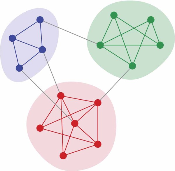
How will we do this? Use the stochastic block model (let's call it SBM) -- we have graphs of $G(n,p,q)$ (for simplicity, let's assume $n$ is even and $p>q$).
In this model, we have two "communities" each of size $\frac{n}{2}$ such that the probability of an edge existing between any two nodes within a community is $p$ and the probability of an edge between the two communities is $q$.

Our goal will be to recover the original communities. For this example, the result would look something like:
 Let's begin by defining a function to generate graphs according to the stochastic block model.
3a. Fill out the following function to create a graph $G(n,p,q)$ according to the SBM.
Important Note: make sure that the first $\frac{n}{2}$ nodes are part of community A and the second $\frac{n}{2}$ nodes are part of community B.
We will be using this assumption for later questions in this lab, when we try to recover the two communities.
def G(n,p,q):
    """
    Let the first n/2 nodes be part of community A and
    the second n/2 part of community B.
    """
    assert(n % 2 == 0)
    assert(p > q)
    mid = int(n/2)
    graph = []
    for i in xrange(n):
        graph.append((i,i))

    #Make community A
    ### Your code here

    #Make community B
    ### Your code here

    #Form connections between communities
    for i in xrange(mid):
        for j in xrange(mid, n):
            if rnd.random() < q:
                graph.append( (i, j) )
    return graph
Let's try testing this out with an example graph -- check that it looks right!
graph = G(20,0.6,0.05)
draw_graph(graph,graph_layout='spring')
Now recall the previous example:
How did we determine the most likely assignment of nodes to communities?
An intuitive approach is to find the min-bisection -- the split of $G$ into 2 groups each of size $\frac{n}{2}$ that has the minimum total edge weight across the partition.
It turns out that this approach is the optimal method of recoverying community assignments in the MAP (maximum a posteriori) sense. (Since each community assignment is equally likely, MAP reduces to MLE (maximum likelihood estimation) in this situation).
In this week's homework you should prove that the likelihood is maximized by minimizing the number of edges across the two partitions.
3b. Given a graph $G(n,p,q)$, write a function to find the maximum likelihood estimate of the two communities.
It might be helpful to have a graph stored as an adjacency list.
from collections import defaultdict

def adjacency_list(graph):
    """
    Takes in the current representation of the graph, outputs an equivalent
    adjacenty list
    """
    adj_list = defaultdict(set)
    for node in graph:
        adj_list[node[0]].add(node[1])
        adj_list[node[1]].add(node[0])
    return adj_list

def mle(graph):
    """
    Return a list of size n/2 that contains the nodes of one of the
    two communities in the graph.

    The other community is implied to be the set of of nodes that
    aren't in the returned result of this function.
    """
    return None
Here's a quick test for your MLE function -- check that the resulting partitions look okay!
graph = G(10,0.6,0.05)
draw_graph(graph,graph_layout='spring')
community = mle(graph)
assert len(community) == 5

print 'The community found is the nodes', community
Now recall that important note from earlier -- in the graphs we generate, the first $\frac{n}{2}$ nodes are from community A and the second $\frac{n}{2}$ nodes from community B.
We can therefore test whether or not our MLE method accurately recovers these two communities from randomly generated graphs that we generate. In this section we will simulate the probability of exact recovery using MLE.
3c. Write a function to simulate the probability of exact recovery through MLE given $n,p,q$.
def prob_recovery(n, alpha, beta):
    """
    Simulate the probability of exact recovery through MLE.
    Use 100 samples.
    """
    mid = int(n/2)
    ground_truth1 = tuple(np.arange(mid))
    ground_truth2 = tuple(np.arange(mid, n))

    ### Your code here
    ### Note that the returned result by mle() should either be ground_truth1 or ground_truth2

    return None
Here's a few examples to test your simulation:
print "P(recovery) for n=10, p=0.6, q=0.05 --", prob_recovery(10, 0.6, 0.05) # usually recovers
print "P(recovery) for n=10, p=0.92, q=0.06 --", prob_recovery(10, 0.92, 0.06)  # almost certainly recovers
print "P(recovery) for n=10, p=0.12, q=0.06 --", prob_recovery(10, 0.12, 0.06)  # almost certainly fails
3d. Can you find a threshold on $(p, q, n)$ for exact recovery through MLE?
It turns out that there is a threshold on $(p,q,n)$ for a phase transition which determines whether or not the communities can be recovered using MLE.
This part of the lab is meant to be open-ended. You should use the code you've already written to help arrive at an expression for threshold in the form
$$f(p,q,n) > 1$$After this threshold, can almost recover the original communities in the SBM.
We will grade this portion leniently and based on the amount of effort put in.
### Your code here
Congratulations! You've reached the end of the lab.
For those who are interested, with the solutions we will release an (optional) lab as reading that guides you through the proof of this threshold in depth. It will also explore more efficient techniques (the MLE technique is NP-hard) to solve the problem of exact recovery.