Decision tree for classification in plain Python
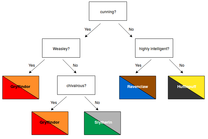
A decision tree is a supervised machine learning model that can be used both for classification and regression. At its core, a decision tree uses a tree structure to predict an output value for a given input example. In the tree, each path from the root node to a leaf node represents a decision path that ends in a predicted value.
A simple example might look as follows:
Decision trees have many advantages. For example, they are easy to understand and their decisions are easy to interpret. Also, they don't require a lot of data preparation. A more extensive list of their advantages and disadvantages can be found here.
CART training algorithm
In order to train a decision tree, various algorithms can be used. In this notebook we will focus on the CART algorithm (Classification and Regression Trees) for classification. The CART algorithm builds a binary tree in which every non-leaf node has exactly two children (corresponding to a yes/no answer).
Given a set of training examples and their labels, the algorithm repeatedly splits the training examples $D$ into two subsets $D_{left}, D_{right}$ using some feature $f$ and feature threshold $t_f$ such that samples with the same label are grouped together. At each node, the algorithm selects the split $\theta = (f, t_f)$ that produces the purest subsets, weighted by their size. Purity/impurity is measured using the Gini impurity.
So at each step, the algorithm selects the parameters $\theta$ that minimize the following cost function:
\begin{equation} J(D, \theta) = \frac{n_{left}}{n_{total}} G_{left} + \frac{n_{right}}{n_{total}} G_{right} \end{equation}- $D$: remaining training examples
- $n_{total}$ : number of remaining training examples
- $\theta = (f, t_f)$: feature and feature threshold
- $n_{left}/n_{right}$: number of samples in the left/right subset
- $G_{left}/G_{right}$: Gini impurity of the left/right subset
This step is repeated recursively until the maximum allowable depth is reached or the current number of samples $n_{total}$ drops below some minimum number. The original equations can be found here.
After building the tree, new examples can be classified by navigating through the tree, testing at each node the corresponding feature until a leaf node/prediction is reached.
Gini Impurity
Given $K$ different classification values $k \in \{1, ..., K\}$ the Gini impurity of node $m$ is computed as follows:
\begin{equation} G_m = 1 - \sum_{k=1}^{K} (p_{m,k})^2 \end{equation}where $p_{m, k}$ is the fraction of training examples with class $k$ among all training examples in node $m$.
The Gini impurity can be used to evaluate how good a potential split is. A split divides a given set of training examples into two groups. Gini measures how "mixed" the resulting groups are. A perfect separation (i.e. each group contains only samples of the same class) corresponds to a Gini impurity of 0. If the resulting groups contain equally many samples of each class, the Gini impurity will reach its highest value of 0.5
Caveats
Without regularization, decision trees are likely to overfit the training examples. This can be prevented using techniques like pruning or by providing a maximum allowed tree depth and/or a minimum number of samples required to split a node further.
from sklearn.datasets import load_iris
import numpy as np
import matplotlib.pyplot as plt
from sklearn.model_selection import train_test_split
np.random.seed(123)

%matplotlib inline
Dataset
The iris dataset compromises 150 examples of 3 different species of iris flowers (Setosa, Versicolour, and Virginica). Each example is described by four attributes: sepal length (cm), sepal width (cm), petal length (cm), petal width (cm).
iris = load_iris()

X, y = iris.data, iris.target
# Split the data into a training and test set
X_train, X_test, y_train, y_test = train_test_split(X, y)

print(f'Shape X_train: {X_train.shape}')
print(f'Shape y_train: {y_train.shape}')
print(f'Shape X_test: {X_test.shape}')
print(f'Shape y_test: {y_test.shape}')
Shape X_train: (112, 4)
Shape y_train: (112,)
Shape X_test: (38, 4)
Shape y_test: (38,)
Decision tree class
Parts of this code were inspired by this tutorial
class DecisionTree:
    """
    Decision tree for classification
    """

    def __init__(self):
        self.root_dict = None
        self.tree_dict = None

    def split_dataset(self, X, y, feature_idx, threshold):
        """
        Splits dataset X into two subsets, according to a given feature
        and feature threshold.

        Args:
            X: 2D numpy array with data samples
            y: 1D numpy array with labels
            feature_idx: int, index of feature used for splitting the data
            threshold: float, threshold used for splitting the data

        Returns:
            splits: dict containing the left and right subsets
            and their labels
        """

        left_idx = np.where(X[:, feature_idx] < threshold)
        right_idx = np.where(X[:, feature_idx] >= threshold)

        left_subset = X[left_idx]
        y_left = y[left_idx]

        right_subset = X[right_idx]
        y_right = y[right_idx]

        splits = {
        'left': left_subset,
        'y_left': y_left,
        'right': right_subset,
        'y_right': y_right,
        }

        return splits

    def gini_impurity(self, y_left, y_right, n_left, n_right):
        """
        Computes Gini impurity of a split.

        Args:
            y_left, y_right: target values of samples in left/right subset
            n_left, n_right: number of samples in left/right subset

        Returns:
            gini_left: float, Gini impurity of left subset
            gini_right: gloat, Gini impurity of right subset
        """

        n_total = n_left + n_left

        score_left, score_right = 0, 0
        gini_left, gini_right = 0, 0

        if n_left != 0:
            for c in range(self.n_classes):
                # For each class c, compute fraction of samples with class c
                p_left = len(np.where(y_left == c)[0]) / n_left
                score_left += p_left * p_left
            gini_left = 1 - score_left

        if n_right != 0:
            for c in range(self.n_classes):
                p_right = len(np.where(y_right == c)[0]) / n_right
                score_right += p_right * p_right
            gini_right = 1 - score_right

        return gini_left, gini_right

    def get_cost(self, splits):
        """
        Computes cost of a split given the Gini impurity of
        the left and right subset and the sizes of the subsets

        Args:
            splits: dict, containing params of current split
        """
        y_left = splits['y_left']
        y_right = splits['y_right']

        n_left = len(y_left)
        n_right = len(y_right)
        n_total = n_left + n_right

        gini_left, gini_right = self.gini_impurity(y_left, y_right, n_left, n_right)
        cost = (n_left / n_total) * gini_left + (n_right / n_total) * gini_right

        return cost

    def find_best_split(self, X, y):
        """
        Finds the best feature and feature index to split dataset X into
        two groups. Checks every value of every attribute as a candidate
        split.

        Args:
            X: 2D numpy array with data samples
            y: 1D numpy array with labels

        Returns:
            best_split_params: dict, containing parameters of the best split
        """

        n_samples, n_features = X.shape

        best_feature_idx, best_threshold, best_cost, best_splits = np.inf, np.inf, np.inf, None

        for feature_idx in range(n_features):
            for i in range(n_samples):
                current_sample = X[i]
                threshold = current_sample[feature_idx]
                splits = self.split_dataset(X, y, feature_idx, threshold)
                cost = self.get_cost(splits)

                if cost < best_cost:
                    best_feature_idx = feature_idx
                    best_threshold = threshold
                    best_cost = cost
                    best_splits = splits

        best_split_params = {
            'feature_idx': best_feature_idx,
            'threshold': best_threshold,
            'cost': best_cost,
            'left': best_splits['left'],
            'y_left': best_splits['y_left'],
            'right': best_splits['right'],
            'y_right': best_splits['y_right'],
        }

        return best_split_params


    def build_tree(self, node_dict, depth, max_depth, min_samples):
        """
        Builds the decision tree in a recursive fashion.

        Args:
            node_dict: dict, representing the current node
            depth: int, depth of current node in the tree
            max_depth: int, maximum allowed tree depth
            min_samples: int, minimum number of samples needed to split a node further

        Returns:
            node_dict: dict, representing the full subtree originating from current node
        """
        left_samples = node_dict['left']
        right_samples = node_dict['right']
        y_left_samples = node_dict['y_left']
        y_right_samples = node_dict['y_right']

        if len(y_left_samples) == 0 or len(y_right_samples) == 0:
            node_dict["left_child"] = node_dict["right_child"] = self.create_terminal_node(np.append(y_left_samples, y_right_samples))
            return None

        if depth >= max_depth:
            node_dict["left_child"] = self.create_terminal_node(y_left_samples)
            node_dict["right_child"] = self.create_terminal_node(y_right_samples)
            return None

        if len(right_samples) < min_samples:
            node_dict["right_child"] = self.create_terminal_node(y_right_samples)
        else:
            node_dict["right_child"] = self.find_best_split(right_samples, y_right_samples)
            self.build_tree(node_dict["right_child"], depth+1, max_depth, min_samples)

        if len(left_samples) < min_samples:
            node_dict["left_child"] = self.create_terminal_node(y_left_samples)
        else:
            node_dict["left_child"] = self.find_best_split(left_samples, y_left_samples)
            self.build_tree(node_dict["left_child"], depth+1, max_depth, min_samples)

        return node_dict

    def create_terminal_node(self, y):
        """
        Creates a terminal node.
        Given a set of labels the most common label is computed and
        set as the classification value of the node.

        Args:
            y: 1D numpy array with labels
        Returns:
            classification: int, predicted class
        """
        classification = max(set(y), key=list(y).count)
        return classification

    def train(self, X, y, max_depth, min_samples):
        """
        Fits decision tree on a given dataset.

        Args:
            X: 2D numpy array with data samples
            y: 1D numpy array with labels
            max_depth: int, maximum allowed tree depth
            min_samples: int, minimum number of samples needed to split a node further
        """
        self.n_classes = len(set(y))
        self.root_dict = self.find_best_split(X, y)
        self.tree_dict = self.build_tree(self.root_dict, 1, max_depth, min_samples)

    def predict(self, X, node):
        """
        Predicts the class for a given input example X.

        Args:
            X: 1D numpy array, input example
            node: dict, representing trained decision tree

        Returns:
            prediction: int, predicted class
        """
        feature_idx = node['feature_idx']
        threshold = node['threshold']

        if X[feature_idx] < threshold:
            if isinstance(node['left_child'], (int, np.integer)):
                return node['left_child']
            else:
                prediction = self.predict(X, node['left_child'])
        elif X[feature_idx] >= threshold:
            if isinstance(node['right_child'], (int, np.integer)):
                return node['right_child']
            else:
                prediction = self.predict(X, node['right_child'])

        return prediction
Initializing and training the decision tree
tree = DecisionTree()
tree.train(X_train, y_train, max_depth=2, min_samples=1)
Printing the decision tree structure
def print_tree(node, depth=0):
    if isinstance(node, (int, np.integer)):
        print(f"{depth * '  '}predicted class: {iris.target_names[node]}")
    else:
        print(f"{depth * '  '}{iris.feature_names[node['feature_idx']]} < {node['threshold']}, "
             f"cost of split: {round(node['cost'], 3)}")
        print_tree(node["left_child"], depth+1)
        print_tree(node["right_child"], depth+1)
print_tree(tree.tree_dict)
petal length (cm) < 3.0, cost of split: 0.346
  sepal length (cm) < 5.4, cost of split: 0.0
    predicted class: setosa
    predicted class: setosa
  petal width (cm) < 1.8, cost of split: 0.097
    predicted class: versicolor
    predicted class: virginica
Testing the decision tree
all_predictions = []
for i in range(X_test.shape[0]):
    result = tree.predict(X_test[i], tree.tree_dict)
    all_predictions.append(y_test[i] == result)

print(f"Accuracy on test set: {sum(all_predictions) / len(all_predictions)}")
Accuracy on test set: 0.9473684210526315