Bayesian Temporal Matrix Factorization
Published: October 8, 2019
Revised: October 8, 2020
Author: Xinyu Chen [GitHub homepage]
Download: This Jupyter notebook is at our GitHub repository. If you want to evaluate the code, please download the notebook from the transdim repository.
This notebook shows how to implement the Bayesian Temporal Matrix Factorization (BTMF), a fully Bayesian matrix factorization model, on some real-world data sets. To overcome the missing data problem in multivariate time series, BTMF takes into account both low-rank matrix structure and time series autoregression. For an in-depth discussion of BTMF, please see [1].
Abstract
Large-scale and multidimensional spatiotemporal data sets are becoming ubiquitous in many real-world applications such as monitoring traffic and air quality. Making predictions on these time series has become a critical challenge due to not only the large-scale and high-dimensional nature but also the considerable amount of missing data. In this work, we propose a Bayesian Temporal Matrix Factorization (BTMF) model for modeling multidimensional time series - and in particular spatiotemporal data - in the presence of missing values. By integrating low-rank matrix factorization and vector autoregressive (VAR) process into a single probabilistic graphical model, our model can effectively perform predictions without imputing those missing values. We develop efficient Gibbs sampling algorithms for model inference and test BTMF on several real-world spatiotemporal data sets (i.e., a typical kind of multivariate time series data) for both missing data imputation and short-term rolling prediction tasks. This post is mainly about BTMF and its Python implementation with an application of spatiotemporal data imputation.
Problem Description
We assume a spatiotemporal setting for multidimensional time series data throughout this work. In general, modern spatiotemporal data sets collected from sensor networks can be organized as matrix time series. For example, we can denote by matrix $Y\in\mathbb{R}^{N\times T}$ a multivariate time series collected from $N$ locations/sensors on $T$ time points, with each row $$\boldsymbol{y}_{i}=\left(y_{i,1},y_{i,2},...,y_{i,t-1},y_{i,t},y_{i,t+1},...,y_{i,T}\right)$$ corresponding to the time series collected at location $i$.
As mentioned, making accurate predictions on incomplete time series is very challenging, while missing data problem is almost inevitable in real-world applications. Figure 1 illustrates the prediction problem for incomplete time series data. Here we use $(i,t)\in\Omega$ to index the observed entries in matrix $Y$.
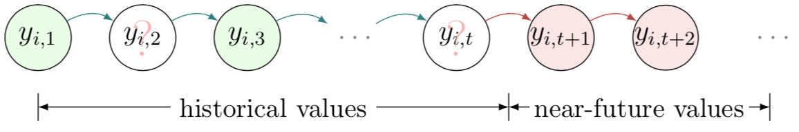
Figure 1: Illustration of multivariate time series and the prediction problem in the presence of missing values (green: observed data; white: missing data; red: prediction).
Model Description
Given a partially observed spatiotemporal matrix $Y\in\mathbb{R}^{N \times T}$, one can factorize it into a spatial factor matrix $W\in\mathbb{R}^{R \times N}$ and a temporal factor matrix $X\in\mathbb{R}^{R \times T}$ following general matrix factorization model: \begin{equation} Y\approx W^{\top}X, \label{btmf_equation1} \end{equation} and element-wise, we have \begin{equation} y_{it}\approx \boldsymbol{w}_{i}^\top\boldsymbol{x}_{t}, \quad \forall (i,t), \label{btmf_equation2} \end{equation} where vectors $\boldsymbol{w}_{i}$ and $\boldsymbol{x}_{t}$ refer to the $i$-th column of $W$ and the $t$-th column of $X$, respectively.
The standard matrix factorization model is a good approach to deal with the missing data problem; however, it cannot capture the dependencies among different columns in $X$, which are critical in modeling time series data. To better characterize the temporal dependencies and impose temporal smoothness, a novel AR regularizer is introduced on $X$ in TRMF (i.e., Temporal Regularizer Matrix Factorization proposed by Yu et al., 2016): \begin{equation} \label{equ:VAR} \begin{aligned} \boldsymbol{x}_{t+1}&=\sum\nolimits_{k=1}^{d}A_{k}\boldsymbol{x}_{t+1-h_k}+\boldsymbol{\epsilon}_t, \\ &=A^\top \boldsymbol{v}_{t+1}+\boldsymbol{\epsilon}_{t}, \\ \end{aligned} \end{equation} where $\mathcal{L}=\left\{h_1,\ldots,h_k,\ldots,h_d\right\}$ is a lag set ($d$ is the order of this AR model), each $A_k$ ($k\in\left\{1,...,d\right\}$) is a $R\times R$ coefficient matrix, and $\boldsymbol{\epsilon}_t$ is a zero mean Gaussian noise vector. For brevity, matrix $A\in \mathbb{R}^{(R d) \times R}$ and vector $\boldsymbol{v}_{t+1}\in \mathbb{R}^{(R d) \times 1}$ are defined as \begin{equation*} A=\left[A_{1}, \ldots, A_{d}\right]^{\top} ,\quad \boldsymbol{v}_{t+1}=\left[\begin{array}{c}{\boldsymbol{x}_{t+1-h_1}} \\ {\vdots} \\ {\boldsymbol{x}_{t+1-h_d}}\end{array}\right] . \end{equation*}

Figure 2: A graphical illustration of the rolling prediction scheme using BTMF (with VAR process) (green: observed data; white: missing data; red: prediction).
In Yu et al., 2016, to avoid overfitting and reduce the number of parameters, the coefficient matrix in TRMF is further assumed to be a diagonal $A_k=\text{diag}(\boldsymbol{\theta}_{k})$. Therefore, they have \begin{equation} \label{equ:AR} \boldsymbol{x}_{t+1}=\boldsymbol{\theta}_{1}\circledast\boldsymbol{x}_{t+1-h_1}+\cdots+\boldsymbol{\theta}_{d}\circledast\boldsymbol{x}_{t+1-h_d}+\boldsymbol{\epsilon}_t, \end{equation} where the symbol $\circledast$ denotes the element-wise Hadamard product. However, unlike this individual autoregressive (AR) process, a vector autoregressive (VAR) process is actually more powerful for capturing multivariate time series patterns.

Figure 3: A graphical illustration of the rolling prediction scheme using BTMF (with AR process) (green: observed data; white: missing data; red: prediction).
Bayesian Temporal Matrix Factorization Model
1 Model Specification
Following the general Bayesian probabilistic matrix factorization models (e.g., BPMF proposed by Salakhutdinov & Mnih, 2008), we assume that each observed entry in $Y$ follows a Gaussian distribution with precision $\tau$: \begin{equation} y_{i,t}\sim\mathcal{N}\left(\boldsymbol{w}_i^\top\boldsymbol{x}_t,\tau^{-1}\right),\quad \left(i,t\right)\in\Omega. \label{btmf_equation3} \end{equation}
On the spatial dimension, we use a simple Gaussian factor matrix without imposing any dependencies explicitly: \begin{equation} \boldsymbol{w}_i\sim\mathcal{N}\left(\boldsymbol{\mu}_{w},\Lambda_w^{-1}\right), \end{equation} and we place a conjugate Gaussian-Wishart prior on the mean vector and the precision matrix: \begin{equation} \boldsymbol{\mu}_w | \Lambda_w \sim\mathcal{N}\left(\boldsymbol{\mu}_0,(\beta_0\Lambda_w)^{-1}\right),\Lambda_w\sim\mathcal{W}\left(W_0,\nu_0\right), \end{equation} where $\boldsymbol{\mu}_0\in \mathbb{R}^{R}$ is a mean vector, $\mathcal{W}\left(W_0,\nu_0\right)$ is a Wishart distribution with a $R\times R$ scale matrix $W_0$ and $\nu_0$ degrees of freedom.
In modeling the temporal factor matrix $X$, we re-write the VAR process as: \begin{equation} \begin{aligned} \boldsymbol{x}_{t}&\sim\begin{cases} \mathcal{N}\left(\boldsymbol{0},I_R\right),&\text{if $t\in\left\{1,2,...,h_d\right\}$}, \\ \mathcal{N}\left(A^\top \boldsymbol{v}_{t},\Sigma\right),&\text{otherwise},\\ \end{cases}\\ \end{aligned} \label{btmf_equation5} \end{equation}
Since the mean vector is defined by VAR, we need to place the conjugate matrix normal inverse Wishart (MNIW) prior on the coefficient matrix $A$ and the covariance matrix $\Sigma$ as follows, \begin{equation} \begin{aligned} A\sim\mathcal{MN}_{(Rd)\times R}\left(M_0,\Psi_0,\Sigma\right),\quad \Sigma \sim\mathcal{IW}\left(S_0,\nu_0\right), \\ \end{aligned} \end{equation} where the probability density function for the $Rd$-by-$R$ random matrix $A$ has the form: \begin{equation} \begin{aligned} &p\left(A\mid M_0,\Psi_0,\Sigma\right) \\ =&\left(2\pi\right)^{-R^2d/2}\left|\Psi_0\right|^{-R/2}\left|\Sigma\right|^{-Rd/2} \\ &\times \exp\left(-\frac{1}{2}\text{tr}\left[\Sigma^{-1}\left(A-M_0\right)^{\top}\Psi_{0}^{-1}\left(A-M_0\right)\right]\right), \\ \end{aligned} \label{mnpdf} \end{equation} where $\Psi_0\in\mathbb{R}^{(Rd)\times (Rd)}$ and $\Sigma\in\mathbb{R}^{R\times R}$ are played as covariance matrices.
For the only remaining parameter $\tau$, we place a Gamma prior $\tau\sim\text{Gamma}\left(\alpha,\beta\right)$ where $\alpha$ and $\beta$ are the shape and rate parameters, respectively.
The above specifies the full generative process of BTMF, and we could also see the Bayesian graphical model shown in Figure 4. Several parameters are introduced to define the prior distributions for hyperparameters, including $\boldsymbol{\mu}_{0}$, $W_0$, $\nu_0$, $\beta_0$, $\alpha$, $\beta$, $M_0$, $\Psi_0$, and $S_0$. These parameters need to provided in advance when training the model. However, it should be noted that the specification of these parameters has little impact on the final results, as the training data will play a much more important role in defining the posteriors of the hyperparameters.

Figure 4: An overview graphical model of BTMF (time lag set: $\left\{1,2,...,d\right\}$). The shaded nodes ($y_{i,t}$) are the observed data in $\Omega$.
2 Model Inference
Given the complex structure of BTMF, it is intractable to write down the posterior distribution. Here we rely on the MCMC technique for Bayesian learning. In detail, we introduce a Gibbs sampling algorithm by deriving the full conditional distributions for all parameters and hyperparameters. Thanks to the use of conjugate priors in Figure 4, we can actually write down all the conditional distributions analytically. Below we summarize the Gibbs sampling procedure.
1) Sampling Factor Matrix $W$ and Its Hyperparameters
For programming convenience, we use $W\in\mathbb{R}^{N\times R}$ to replace $W\in\mathbb{R}^{R\times N}$.
import numpy as np
from numpy.linalg import inv as inv
from numpy.random import normal as normrnd
from scipy.linalg import khatri_rao as kr_prod
from scipy.stats import wishart
from scipy.stats import invwishart
from numpy.linalg import solve as solve
from numpy.linalg import cholesky as cholesky_lower
from scipy.linalg import cholesky as cholesky_upper
from scipy.linalg import solve_triangular as solve_ut
import matplotlib.pyplot as plt
%matplotlib inline
def mvnrnd_pre(mu, Lambda):
    src = normrnd(size = (mu.shape[0],))
    return solve_ut(cholesky_upper(Lambda, overwrite_a = True, check_finite = False),
                    src, lower = False, check_finite = False, overwrite_b = True) + mu

def cov_mat(mat, mat_bar):
    mat = mat - mat_bar
    return mat.T @ mat
def sample_factor_w(tau_sparse_mat, tau_ind, W, X, tau, beta0 = 1, vargin = 0):
    """Sampling N-by-R factor matrix W and its hyperparameters (mu_w, Lambda_w)."""

    dim1, rank = W.shape
    W_bar = np.mean(W, axis = 0)
    temp = dim1 / (dim1 + beta0)
    var_W_hyper = inv(np.eye(rank) + cov_mat(W, W_bar) + temp * beta0 * np.outer(W_bar, W_bar))
    var_Lambda_hyper = wishart.rvs(df = dim1 + rank, scale = var_W_hyper)
    var_mu_hyper = mvnrnd_pre(temp * W_bar, (dim1 + beta0) * var_Lambda_hyper)

    if dim1 * rank ** 2 > 1e+8:
        vargin = 1

    if vargin == 0:
        var1 = X.T
        var2 = kr_prod(var1, var1)
        var3 = (var2 @ tau_ind.T).reshape([rank, rank, dim1]) + var_Lambda_hyper[:, :, None]
        var4 = var1 @ tau_sparse_mat.T + (var_Lambda_hyper @ var_mu_hyper)[:, None]
        for i in range(dim1):
            W[i, :] = mvnrnd_pre(solve(var3[:, :, i], var4[:, i]), var3[:, :, i])
    elif vargin == 1:
        for i in range(dim1):
            pos0 = np.where(sparse_mat[i, :] != 0)
            Xt = X[pos0[0], :]
            var_mu = tau[i] * Xt.T @ sparse_mat[i, pos0[0]] + var_Lambda_hyper @ var_mu_hyper
            var_Lambda = tau[i] * Xt.T @ Xt + var_Lambda_hyper
            W[i, :] = mvnrnd_pre(solve(var_Lambda, var_mu), var_Lambda)

    return W
2) Sampling VAR Coefficients $A$ and Its Hyperparameters
Foundations of VAR
Vector autoregression (VAR) is a multivariate extension of autoregression (AR). Formally, VAR for $R$-dimensional vectors $\boldsymbol{x}_{t}$ can be written as follows, \begin{equation} \begin{aligned} \boldsymbol{x}_{t}&=A_{1} \boldsymbol{x}_{t-h_1}+\cdots+A_{d} \boldsymbol{x}_{t-h_d}+\boldsymbol{\epsilon}_{t}, \\ &= A^\top \boldsymbol{v}_{t}+\boldsymbol{\epsilon}_{t},~t=h_d+1, \ldots, T, \\ \end{aligned} \end{equation} where \begin{equation} A=\left[A_{1}, \ldots, A_{d}\right]^{\top} \in \mathbb{R}^{(R d) \times R},\quad \boldsymbol{v}_{t}=\left[\begin{array}{c}{\boldsymbol{x}_{t-h_1}} \\ {\vdots} \\ {\boldsymbol{x}_{t-h_d}}\end{array}\right] \in \mathbb{R}^{(R d) \times 1}. \end{equation}
In the following, if we define \begin{equation} Z=\left[\begin{array}{c}{\boldsymbol{x}_{h_d+1}^{\top}} \\ {\vdots} \\ {\boldsymbol{x}_{T}^{\top}}\end{array}\right] \in \mathbb{R}^{(T-h_d) \times R},\quad Q=\left[\begin{array}{c}{\boldsymbol{v}_{h_d+1}^{\top}} \\ {\vdots} \\ {\boldsymbol{v}_{T}^{\top}}\end{array}\right] \in \mathbb{R}^{(T-h_d) \times(R d)}, \end{equation} then, we could write the above mentioned VAR as \begin{equation} \underbrace{Z}_{(T-h_d)\times R}\approx \underbrace{Q}_{(T-h_d)\times (Rd)}\times \underbrace{A}_{(Rd)\times R}. \end{equation}
To include temporal factors $\boldsymbol{x}_{t},t=1,...,h_d$, we also define $$Z_0=\left[\begin{array}{c}{\boldsymbol{x}_{1}^{\top}} \\ {\vdots} \\ {\boldsymbol{x}_{h_d}^{\top}}\end{array}\right] \in \mathbb{R}^{h_d \times R}.$$
Build a Bayesian VAR on temporal factors $\boldsymbol{x}_{t}$ \begin{equation} \begin{aligned} \boldsymbol{x}_{t}&\sim\begin{cases}\mathcal{N}\left(A^\top \boldsymbol{v}_{t},\Sigma\right),~\text{if $t\in\left\{h_d+1,...,T\right\}$},\\{\mathcal{N}\left(\boldsymbol{0},I_R\right),~\text{otherwise}}.\end{cases}\\ A&\sim\mathcal{MN}_{(Rd)\times R}\left(M_0,\Psi_0,\Sigma\right), \\ \Sigma &\sim\mathcal{IW}\left(S_0,\nu_0\right), \\ \end{aligned} \end{equation} where \begin{equation} \begin{aligned} &\mathcal{M N}_{(R d) \times R}\left(A | M_{0}, \Psi_{0}, \Sigma\right)\\ \propto|&\Sigma|^{-R d / 2} \exp \left(-\frac{1}{2} \operatorname{tr}\left[\Sigma^{-1}\left(A-M_{0}\right)^{\top} \Psi_{0}^{-1}\left(A-M_{0}\right)\right]\right), \\ \end{aligned} \end{equation} and \begin{equation} \mathcal{I} \mathcal{W}\left(\Sigma | S_{0}, \nu_{0}\right) \propto|\Sigma|^{-\left(\nu_{0}+R+1\right) / 2} \exp \left(-\frac{1}{2} \operatorname{tr}\left(\Sigma^{-1}S_{0}\right)\right). \end{equation}
Likelihood from temporal factors $\boldsymbol{x}_{t}$ \begin{equation} \begin{aligned} &\mathcal{L}\left(X\mid A,\Sigma\right) \\ \propto &\prod_{t=1}^{h_d}p\left(\boldsymbol{x}_{t}\mid \Sigma\right)\times \prod_{t=h_d+1}^{T}p\left(\boldsymbol{x}_{t}\mid A,\Sigma\right) \\ \propto &\left|\Sigma\right|^{-T/2}\exp\left\{-\frac{1}{2}\sum_{t=h_d+1}^{T}\left(\boldsymbol{x}_{t}-A^\top \boldsymbol{v}_{t}\right)^\top\Sigma^{-1}\left(\boldsymbol{x}_{t}-A^\top \boldsymbol{v}_{t}\right)\right\} \\ \propto &\left|\Sigma\right|^{-T/2}\exp\left\{-\frac{1}{2}\text{tr}\left[\Sigma^{-1}\left(Z_0^\top Z_0+\left(Z-QA\right)^\top \left(Z-QA\right)\right)\right]\right\} \end{aligned} \end{equation}
Posterior distribution
Consider \begin{equation} \begin{aligned} &\left(A-M_{0}\right)^{\top} \Psi_{0}^{-1}\left(A-M_{0}\right)+S_0+Z_0^\top Z_0+\left(Z-QA\right)^\top \left(Z-QA\right) \\ =&A^\top\left(\Psi_0^{-1}+Q^\top Q\right)A-A^\top\left(\Psi_0^{-1}M_0+Q^\top Z\right) \\ &-\left(\Psi_0^{-1}M_0+Q^\top Z\right)^\top A \\ &+\left(\Psi_0^{-1}M_0+Q^\top Z\right)^\top\left(\Psi_0^{-1}+Q^\top Q\right)\left(\Psi_0^{-1}M_0+Q^\top Z\right) \\ &-\left(\Psi_0^{-1}M_0+Q^\top Z\right)^\top\left(\Psi_0^{-1}+Q^\top Q\right)\left(\Psi_0^{-1}M_0+Q^\top Z\right) \\ &+M_0^\top\Psi_0^{-1}M_0+S_0+Z_0^\top Z_0+Z^\top Z \\ =&\left(A-M^{*}\right)^\top\left(\Psi^{*}\right)^{-1}\left(A-M^{*}\right)+S^{*}, \\ \end{aligned} \end{equation} which is in the form of $\mathcal{MN}\left(\cdot\right)$ and $\mathcal{IW}\left(\cdot\right)$.
The $Rd$-by-$R$ matrix $A$ has a matrix normal distribution, and $R$-by-$R$ covariance matrix $\Sigma$ has an inverse Wishart distribution, that is, \begin{equation} A \sim \mathcal{M N}_{(R d) \times R}\left(M^{*}, \Psi^{*}, \Sigma\right), \quad \Sigma \sim \mathcal{I} \mathcal{W}\left(S^{*}, \nu^{*}\right), \end{equation} with \begin{equation} \begin{cases} {\Psi^{*}=\left(\Psi_{0}^{-1}+Q^{\top} Q\right)^{-1}}, \\ {M^{*}=\Psi^{*}\left(\Psi_{0}^{-1} M_{0}+Q^{\top} Z\right)}, \\ {S^{*}=S_{0}+Z^\top Z+M_0^\top\Psi_0^{-1}M_0-\left(M^{*}\right)^\top\left(\Psi^{*}\right)^{-1}M^{*}}, \\ {\nu^{*}=\nu_{0}+T-h_d}. \end{cases} \end{equation}
def mnrnd(M, U, V):
    """
    Generate matrix normal distributed random matrix.
    M is a m-by-n matrix, U is a m-by-m matrix, and V is a n-by-n matrix.
    """
    dim1, dim2 = M.shape
    X0 = np.random.randn(dim1, dim2)
    P = cholesky_lower(U)
    Q = cholesky_lower(V)

    return M + P @ X0 @ Q.T

def sample_var_coefficient(X, time_lags):
    dim, rank = X.shape
    d = time_lags.shape[0]
    tmax = np.max(time_lags)

    Z_mat = X[tmax : dim, :]
    Q_mat = np.zeros((dim - tmax, rank * d))
    for k in range(d):
        Q_mat[:, k * rank : (k + 1) * rank] = X[tmax - time_lags[k] : dim - time_lags[k], :]
    var_Psi0 = np.eye(rank * d) + Q_mat.T @ Q_mat
    var_Psi = inv(var_Psi0)
    var_M = var_Psi @ Q_mat.T @ Z_mat
    var_S = np.eye(rank) + Z_mat.T @ Z_mat - var_M.T @ var_Psi0 @ var_M
    Sigma = invwishart.rvs(df = rank + dim - tmax, scale = var_S)

    return mnrnd(var_M, var_Psi, Sigma), Sigma
3) Sampling Factor Matrix $X$
Posterior distribution \begin{equation} \begin{aligned} y_{it}&\sim\mathcal{N}\left(\boldsymbol{w}_{i}^\top\boldsymbol{x}_{t},\tau^{-1}\right),~\left(i,t\right)\in\Omega, \\ \boldsymbol{x}_{t}&\sim\begin{cases}\mathcal{N}\left(\sum_{k=1}^{d}A_{k} \boldsymbol{x}_{t-h_k},\Sigma\right),~\text{if $t\in\left\{h_d+1,...,T\right\}$},\\{\mathcal{N}\left(\boldsymbol{0},I\right),~\text{otherwise}}.\end{cases}\\ \end{aligned} \end{equation}
If $t\in\left\{1,...,h_d\right\}$, parameters of the posterior distribution $\mathcal{N}\left(\boldsymbol{x}_{t}\mid \boldsymbol{\mu}_{t}^{*},\Sigma_{t}^{*}\right)$ are \begin{equation} \begin{aligned} \Sigma_{t}^{*}&=\left(\sum_{k=1, h_{d}<t+h_{k} \leq T}^{d} {A}_{k}^{\top} \Sigma^{-1} A_{k}+\tau\sum_{i:(i,t)\in\Omega}\boldsymbol{w}_{i}\boldsymbol{w}_{i}^\top+I\right)^{-1}, \\ \boldsymbol{\mu}_{t}^{*}&=\Sigma_{t}^{*}\left(\sum_{k=1, h_{d}<t+h_{k} \leq T}^{d} A_{k}^{\top} \Sigma^{-1} \boldsymbol{\psi}_{t+h_{k}}+\tau\sum_{i:(i,t)\in\Omega}\boldsymbol{w}_{i}y_{it}\right). \\ \end{aligned} \end{equation}
If $t\in\left\{h_d+1,...,T\right\}$, then parameters of the posterior distribution $\mathcal{N}\left(\boldsymbol{x}_{t}\mid \boldsymbol{\mu}_{t}^{*},\Sigma_{t}^{*}\right)$ are \begin{equation} \begin{aligned} \Sigma_{t}^{*}&=\left(\sum_{k=1, h_{d}<t+h_{k} \leq T}^{d} {A}_{k}^{\top} \Sigma^{-1} A_{k}+\tau\sum_{i:(i,t)\in\Omega}\boldsymbol{w}_{i}\boldsymbol{w}_{i}^\top+\Sigma^{-1}\right)^{-1}, \\ \boldsymbol{\mu}_{t}^{*}&=\Sigma_{t}^{*}\left(\sum_{k=1, h_{d}<t+h_{k} \leq T}^{d} A_{k}^{\top} \Sigma^{-1} \boldsymbol{\psi}_{t+h_{k}}+\tau\sum_{i:(i,t)\in\Omega}\boldsymbol{w}_{i}y_{it}+\Sigma^{-1}\sum_{k=1}^{d}A_{k}\boldsymbol{x}_{t-h_k}\right), \\ \end{aligned} \end{equation} where $$\boldsymbol{\psi}_{t+h_k}=\boldsymbol{x}_{t+h_k}-\sum_{l=1,l\neq k}^{d}A_{l}\boldsymbol{x}_{t+h_k-h_l}.$$
def sample_factor_x(tau_sparse_mat, tau_ind, time_lags, W, X, A, Lambda_x):
    """Sampling T-by-R factor matrix X."""

    dim2, rank = X.shape
    tmax = np.max(time_lags)
    tmin = np.min(time_lags)
    d = time_lags.shape[0]
    A0 = np.dstack([A] * d)
    for k in range(d):
        A0[k * rank : (k + 1) * rank, :, k] = 0
    mat0 = Lambda_x @ A.T
    mat1 = np.einsum('kij, jt -> kit', A.reshape([d, rank, rank]), Lambda_x)
    mat2 = np.einsum('kit, kjt -> ij', mat1, A.reshape([d, rank, rank]))

    var1 = W.T
    var2 = kr_prod(var1, var1)
    var3 = (var2 @ tau_ind).reshape([rank, rank, dim2]) + Lambda_x[:, :, None]
    var4 = var1 @ tau_sparse_mat
    for t in range(dim2):
        Mt = np.zeros((rank, rank))
        Nt = np.zeros(rank)
        Qt = mat0 @ X[t - time_lags, :].reshape(rank * d)
        index = list(range(0, d))
        if t >= dim2 - tmax and t < dim2 - tmin:
            index = list(np.where(t + time_lags < dim2))[0]
        elif t < tmax:
            Qt = np.zeros(rank)
            index = list(np.where(t + time_lags >= tmax))[0]
        if t < dim2 - tmin:
            Mt = mat2.copy()
            temp = np.zeros((rank * d, len(index)))
            n = 0
            for k in index:
                temp[:, n] = X[t + time_lags[k] - time_lags, :].reshape(rank * d)
                n += 1
            temp0 = X[t + time_lags[index], :].T - np.einsum('ijk, ik -> jk', A0[:, :, index], temp)
            Nt = np.einsum('kij, jk -> i', mat1[index, :, :], temp0)

        var3[:, :, t] = var3[:, :, t] + Mt
        if t < tmax:
            var3[:, :, t] = var3[:, :, t] - Lambda_x + np.eye(rank)
        X[t, :] = mvnrnd_pre(solve(var3[:, :, t], var4[:, t] + Nt + Qt), var3[:, :, t])

    return X
4) Sampling Precision $\tau$
def sample_precision_tau(sparse_mat, mat_hat, ind):
    var_alpha = 1e-6 + 0.5 * np.sum(ind, axis = 1)
    var_beta = 1e-6 + 0.5 * np.sum(((sparse_mat - mat_hat) ** 2) * ind, axis = 1)
    return np.random.gamma(var_alpha, 1 / var_beta)

def sample_precision_scalar_tau(sparse_mat, mat_hat, ind):
    var_alpha = 1e-6 + 0.5 * np.sum(ind)
    var_beta = 1e-6 + 0.5 * np.sum(((sparse_mat - mat_hat) ** 2) * ind)
    return np.random.gamma(var_alpha, 1 / var_beta)
def compute_mape(var, var_hat):
    return np.sum(np.abs(var - var_hat) / var) / var.shape[0]

def compute_rmse(var, var_hat):
    return  np.sqrt(np.sum((var - var_hat) ** 2) / var.shape[0])
5) BTMF Implementation
def BTMF(dense_mat, sparse_mat, init, rank, time_lags, burn_iter, gibbs_iter, option = "factor"):
    """Bayesian Temporal Matrix Factorization, BTMF."""

    dim1, dim2 = sparse_mat.shape
    d = time_lags.shape[0]
    W = init["W"]
    X = init["X"]
    if np.isnan(sparse_mat).any() == False:
        ind = sparse_mat != 0
        pos_obs = np.where(ind)
        pos_test = np.where((dense_mat != 0) & (sparse_mat == 0))
    elif np.isnan(sparse_mat).any() == True:
        pos_test = np.where((dense_mat != 0) & (np.isnan(sparse_mat)))
        ind = ~np.isnan(sparse_mat)
        pos_obs = np.where(ind)
        sparse_mat[np.isnan(sparse_mat)] = 0
    dense_test = dense_mat[pos_test]
    del dense_mat
    tau = np.ones(dim1)
    W_plus = np.zeros((dim1, rank))
    X_plus = np.zeros((dim2, rank))
    A_plus = np.zeros((rank * d, rank))
    temp_hat = np.zeros(len(pos_test[0]))
    show_iter = 200
    mat_hat_plus = np.zeros((dim1, dim2))
    for it in range(burn_iter + gibbs_iter):
        tau_ind = tau[:, None] * ind
        tau_sparse_mat = tau[:, None] * sparse_mat
        W = sample_factor_w(tau_sparse_mat, tau_ind, W, X, tau)
        A, Sigma = sample_var_coefficient(X, time_lags)
        X = sample_factor_x(tau_sparse_mat, tau_ind, time_lags, W, X, A, inv(Sigma))
        mat_hat = W @ X.T
        if option == "factor":
            tau = sample_precision_tau(sparse_mat, mat_hat, ind)
        elif option == "pca":
            tau = sample_precision_scalar_tau(sparse_mat, mat_hat, ind)
            tau = tau * np.ones(dim1)
        temp_hat += mat_hat[pos_test]
        if (it + 1) % show_iter == 0 and it < burn_iter:
            temp_hat = temp_hat / show_iter
            print('Iter: {}'.format(it + 1))
            print('MAPE: {:.6}'.format(compute_mape(dense_test, temp_hat)))
            print('RMSE: {:.6}'.format(compute_rmse(dense_test, temp_hat)))
            temp_hat = np.zeros(len(pos_test[0]))
            print()
        if it + 1 > burn_iter:
            W_plus += W
            X_plus += X
            A_plus += A
            mat_hat_plus += mat_hat
    mat_hat = mat_hat_plus / gibbs_iter
    W = W_plus / gibbs_iter
    X = X_plus / gibbs_iter
    A = A_plus / gibbs_iter
    print('Imputation MAPE: {:.6}'.format(compute_mape(dense_test, mat_hat[:, : dim2][pos_test])))
    print('Imputation RMSE: {:.6}'.format(compute_rmse(dense_test, mat_hat[:, : dim2][pos_test])))
    print()
    mat_hat[mat_hat < 0] = 0

    return mat_hat, W, X, A
Evaluation on Guangzhou Speed Data
Scenario setting:
- Tensor size: $214\times 61\times 144$ (road segment, day, time of day)
- Non-random missing (NM)
- 40% missing rate
import time
import scipy.io
import numpy as np
np.random.seed(1000)

dense_tensor = scipy.io.loadmat('../datasets/Guangzhou-data-set/tensor.mat')['tensor']
dim = dense_tensor.shape
missing_rate = 0.4 # Non-random missing (NM)
sparse_tensor = dense_tensor * np.round(np.random.rand(dim[0], dim[1])[:, :, np.newaxis] + 0.5 - missing_rate)
dense_mat = dense_tensor.reshape([dim[0], dim[1] * dim[2]])
sparse_mat = sparse_tensor.reshape([dim[0], dim[1] * dim[2]])
del dense_tensor, sparse_tensor
Model setting:
- Low rank: 10
- Time lags: {1, 2, 144}
- The number of burn-in iterations: 1000
- The number of Gibbs iterations: 200
import time
start = time.time()
dim1, dim2 = sparse_mat.shape
rank = 10
time_lags = np.array([1, 2, 144])
init = {"W": 0.01 * np.random.randn(dim1, rank), "X": 0.01 * np.random.randn(dim2, rank)}
burn_iter = 1000
gibbs_iter = 200
mat_hat, W, X, A = BTMF(dense_mat, sparse_mat, init, rank, time_lags, burn_iter, gibbs_iter)
end = time.time()
print('Running time: %d seconds'%(end - start))
Iter: 200
MAPE: 0.104269
RMSE: 4.36081

Iter: 400
MAPE: 0.101626
RMSE: 4.30256

Iter: 600
MAPE: 0.101615
RMSE: 4.3037

Iter: 800
MAPE: 0.101683
RMSE: 4.30592

Iter: 1000
MAPE: 0.101673
RMSE: 4.30681

Imputation MAPE: 0.101755
Imputation RMSE: 4.30853

Running time: 933 seconds
Scenario setting:
- Tensor size: $214\times 61\times 144$ (road segment, day, time of day)
- Random missing (RM)
- 40% missing rate
import time
import scipy.io
import numpy as np
np.random.seed(1000)

dense_tensor = scipy.io.loadmat('../datasets/Guangzhou-data-set/tensor.mat')['tensor']
dim = dense_tensor.shape
missing_rate = 0.4 # Random missing (RM)
sparse_tensor = dense_tensor * np.round(np.random.rand(dim[0], dim[1], dim[2]) + 0.5 - missing_rate)
dense_mat = dense_tensor.reshape([dim[0], dim[1] * dim[2]])
sparse_mat = sparse_tensor.reshape([dim[0], dim[1] * dim[2]])
del dense_tensor, sparse_tensor
Model setting:
- Low rank: 80
- Time lags: {1, 2, 144}
- The number of burn-in iterations: 1000
- The number of Gibbs iterations: 200
import time
start = time.time()
dim1, dim2 = sparse_mat.shape
rank = 80
time_lags = np.array([1, 2, 144])
init = {"W": 0.1 * np.random.randn(dim1, rank), "X": 0.1 * np.random.randn(dim2, rank)}
burn_iter = 1000
gibbs_iter = 200
mat_hat, W, X, A = BTMF(dense_mat, sparse_mat, init, rank, time_lags, burn_iter, gibbs_iter)
end = time.time()
print('Running time: %d seconds'%(end - start))
Iter: 200
MAPE: 0.0778319
RMSE: 3.33635

Iter: 400
MAPE: 0.0768004
RMSE: 3.31004

Iter: 600
MAPE: 0.0764412
RMSE: 3.30118

Iter: 800
MAPE: 0.076182
RMSE: 3.29244

Iter: 1000
MAPE: 0.0761008
RMSE: 3.29149

Imputation MAPE: 0.0760784
Imputation RMSE: 3.29119

Running time: 6351 seconds
Scenario setting:
- Tensor size: $214\times 61\times 144$ (road segment, day, time of day)
- Random missing (RM)
- 60% missing rate
import time
import scipy.io
import numpy as np
np.random.seed(1000)

dense_tensor = scipy.io.loadmat('../datasets/Guangzhou-data-set/tensor.mat')['tensor']
dim = dense_tensor.shape
missing_rate = 0.6 # Random missing (RM)
sparse_tensor = dense_tensor * np.round(np.random.rand(dim[0], dim[1], dim[2]) + 0.5 - missing_rate)
dense_mat = dense_tensor.reshape([dim[0], dim[1] * dim[2]])
sparse_mat = sparse_tensor.reshape([dim[0], dim[1] * dim[2]])
del dense_tensor, sparse_tensor
Model setting:
- Low rank: 80
- Time lags: {1, 2, 144}
- The number of burn-in iterations: 1000
- The number of Gibbs iterations: 200
import time
start = time.time()
dim1, dim2 = sparse_mat.shape
rank = 80
time_lags = np.array([1, 2, 144])
init = {"W": 0.1 * np.random.randn(dim1, rank), "X": 0.1 * np.random.randn(dim2, rank)}
burn_iter = 1000
gibbs_iter = 200
mat_hat, W, X, A = BTMF(dense_mat, sparse_mat, init, rank, time_lags, burn_iter, gibbs_iter)
end = time.time()
print('Running time: %d seconds'%(end - start))
Iter: 200
MAPE: 0.0842265
RMSE: 3.59357

Iter: 400
MAPE: 0.0831631
RMSE: 3.55573

Iter: 600
MAPE: 0.0826056
RMSE: 3.53509

Iter: 800
MAPE: 0.0822812
RMSE: 3.52181

Iter: 1000
MAPE: 0.0820294
RMSE: 3.51294

Imputation MAPE: 0.0819592
Imputation RMSE: 3.51001

Running time: 6355 seconds
Evaluation on Birmingham Parking Data
Scenario setting:
- Tensor size: $30\times 77\times 18$ (parking slot, day, time of day)
- Non-random missing (NM)
- 40% missing rate
import time
import scipy.io
import numpy as np
np.random.seed(1000)

dense_tensor = scipy.io.loadmat('../datasets/Birmingham-data-set/tensor.mat')['tensor']
dim = dense_tensor.shape
missing_rate = 0.4 # Non-random missing (NM)
sparse_tensor = dense_tensor * np.round(np.random.rand(dim[0], dim[1])[:, :, np.newaxis] + 0.5 - missing_rate)
dense_mat = dense_tensor.reshape([dim[0], dim[1] * dim[2]])
sparse_mat = sparse_tensor.reshape([dim[0], dim[1] * dim[2]])
del dense_tensor, sparse_tensor
Model setting:
- Low rank: 20
- Time lags: {1, 2, 18}
- The number of burn-in iterations: 1000
- The number of Gibbs iterations: 200
import time
start = time.time()
dim1, dim2 = sparse_mat.shape
rank = 20
time_lags = np.array([1, 2, 18])
init = {"W": 0.01 * np.random.randn(dim1, rank), "X": 0.01 * np.random.randn(dim2, rank)}
burn_iter = 1000
gibbs_iter = 200
mat_hat, W, X, A = BTMF(dense_mat, sparse_mat, init, rank, time_lags, burn_iter, gibbs_iter)
end = time.time()
print('Running time: %d seconds'%(end - start))
Iter: 200
MAPE: 0.160954
RMSE: 99.1409

Iter: 400
MAPE: 0.130435
RMSE: 80.5966

Iter: 600
MAPE: 0.133369
RMSE: 80.2392

Iter: 800
MAPE: 0.127632
RMSE: 77.7049

Iter: 1000
MAPE: 0.133299
RMSE: 74.0348

Imputation MAPE: 0.13379
Imputation RMSE: 69.5338

Running time: 204 seconds
Scenario setting:
- Tensor size: $30\times 77\times 18$ (parking slot, day, time of day)
- Random missing (RM)
- 40% missing rate
import time
import scipy.io
import numpy as np
np.random.seed(1000)

dense_tensor = scipy.io.loadmat('../datasets/Birmingham-data-set/tensor.mat')['tensor']
dim = dense_tensor.shape
missing_rate = 0.4 # Random missing (RM)
sparse_tensor = dense_tensor * np.round(np.random.rand(dim[0], dim[1], dim[2]) + 0.5 - missing_rate)
dense_mat = dense_tensor.reshape([dim[0], dim[1] * dim[2]])
sparse_mat = sparse_tensor.reshape([dim[0], dim[1] * dim[2]])
del dense_tensor, sparse_tensor
Model setting:
- Low rank: 20
- Time lags: {1, 2, 18}
- The number of burn-in iterations: 1000
- The number of Gibbs iterations: 200
import time
start = time.time()
dim1, dim2 = sparse_mat.shape
rank = 20
time_lags = np.array([1, 2, 18])
init = {"W": 0.1 * np.random.randn(dim1, rank), "X": 0.1 * np.random.randn(dim2, rank)}
burn_iter = 1000
gibbs_iter = 200
mat_hat, W, X, A = BTMF(dense_mat, sparse_mat, init, rank, time_lags, burn_iter, gibbs_iter)
end = time.time()
print('Running time: %d seconds'%(end - start))
Iter: 200
MAPE: 0.0437143
RMSE: 21.7522

Iter: 400
MAPE: 0.0356367
RMSE: 17.9024

Iter: 600
MAPE: 0.0345634
RMSE: 17.0658

Iter: 800
MAPE: 0.0340878
RMSE: 16.2093

Iter: 1000
MAPE: 0.0347393
RMSE: 16.63

Imputation MAPE: 0.0343784
Imputation RMSE: 18.1942

Running time: 204 seconds
Scenario setting:
- Tensor size: $30\times 77\times 18$ (parking slot, day, time of day)
- Random missing (RM)
- 60% missing rate
import time
import scipy.io
import numpy as np
np.random.seed(1000)

dense_tensor = scipy.io.loadmat('../datasets/Birmingham-data-set/tensor.mat')['tensor']
dim = dense_tensor.shape
missing_rate = 0.6 # Random missing (RM)
sparse_tensor = dense_tensor * np.round(np.random.rand(dim[0], dim[1], dim[2]) + 0.5 - missing_rate)
dense_mat = dense_tensor.reshape([dim[0], dim[1] * dim[2]])
sparse_mat = sparse_tensor.reshape([dim[0], dim[1] * dim[2]])
del dense_tensor, sparse_tensor
Model setting:
- Low rank: 20
- Time lags: {1, 2, 18}
- The number of burn-in iterations: 1000
- The number of Gibbs iterations: 200
import time
start = time.time()
dim1, dim2 = sparse_mat.shape
rank = 20
time_lags = np.array([1, 2, 18])
init = {"W": 0.1 * np.random.randn(dim1, rank), "X": 0.1 * np.random.randn(dim2, rank)}
burn_iter = 1000
gibbs_iter = 200
mat_hat, W, X, A = BTMF(dense_mat, sparse_mat, init, rank, time_lags, burn_iter, gibbs_iter)
end = time.time()
print('Running time: %d seconds'%(end - start))
Iter: 200
MAPE: 0.0832529
RMSE: 64.7848

Iter: 400
MAPE: 0.0700006
RMSE: 33.6699

Iter: 600
MAPE: 0.0663554
RMSE: 27.0075

Iter: 800
MAPE: 0.0629423
RMSE: 26.593

Iter: 1000
MAPE: 0.0619536
RMSE: 27.0718

Imputation MAPE: 0.0616117
Imputation RMSE: 25.9018

Running time: 204 seconds
Evaluation on Hangzhou Flow Data
Scenario setting:
- Tensor size: $80\times 25\times 108$ (metro station, day, time of day)
- Non-random missing (NM)
- 40% missing rate
import time
import scipy.io
import numpy as np
np.random.seed(1000)

dense_tensor = scipy.io.loadmat('../datasets/Hangzhou-data-set/tensor.mat')['tensor']
dim = dense_tensor.shape
missing_rate = 0.4 # Non-random missing (NM)
sparse_tensor = dense_tensor * np.round(np.random.rand(dim[0], dim[1])[:, :, np.newaxis] + 0.5 - missing_rate)
dense_mat = dense_tensor.reshape([dim[0], dim[1] * dim[2]])
sparse_mat = sparse_tensor.reshape([dim[0], dim[1] * dim[2]])
del dense_tensor, sparse_tensor
Model setting:
- Low rank: 30
- Time lags: {1, 2, 108}
- The number of burn-in iterations: 1000
- The number of Gibbs iterations: 200
import time
start = time.time()
dim1, dim2 = sparse_mat.shape
rank = 30
time_lags = np.array([1, 2, 108])
init = {"W": 0.01 * np.random.randn(dim1, rank), "X": 0.01 * np.random.randn(dim2, rank)}
burn_iter = 1000
gibbs_iter = 200
mat_hat, W, X, A = BTMF(dense_mat, sparse_mat, init, rank, time_lags, burn_iter, gibbs_iter, option = "pca")
end = time.time()
print('Running time: %d seconds'%(end - start))
Iter: 200
MAPE: 0.280562
RMSE: 103.909

Iter: 400
MAPE: 0.27785
RMSE: 84.921

Iter: 600
MAPE: 0.267921
RMSE: 68.0001

Iter: 800
MAPE: 0.258384
RMSE: 58.105

Iter: 1000
MAPE: 0.259447
RMSE: 48.4835

Imputation MAPE: 0.259309
Imputation RMSE: 46.0055

Running time: 626 seconds
Scenario setting:
- Tensor size: $80\times 25\times 108$ (metro station, day, time of day)
- Random missing (RM)
- 40% missing rate
import time
import scipy.io
import numpy as np
np.random.seed(1000)

dense_tensor = scipy.io.loadmat('../datasets/Hangzhou-data-set/tensor.mat')['tensor']
dim = dense_tensor.shape
missing_rate = 0.4 # Random missing (RM)
sparse_tensor = dense_tensor * np.round(np.random.rand(dim[0], dim[1], dim[2]) + 0.5 - missing_rate)
dense_mat = dense_tensor.reshape([dim[0], dim[1] * dim[2]])
sparse_mat = sparse_tensor.reshape([dim[0], dim[1] * dim[2]])
del dense_tensor, sparse_tensor
Model setting:
- Low rank: 30
- Time lags: {1, 2, 108}
- The number of burn-in iterations: 1000
- The number of Gibbs iterations: 200
import time
start = time.time()
dim1, dim2 = sparse_mat.shape
rank = 30
time_lags = np.array([1, 2, 108])
init = {"W": 0.1 * np.random.randn(dim1, rank), "X": 0.1 * np.random.randn(dim2, rank)}
burn_iter = 1000
gibbs_iter = 200
mat_hat, W, X, A = BTMF(dense_mat, sparse_mat, init, rank, time_lags, burn_iter, gibbs_iter, option = "pca")
end = time.time()
print('Running time: %d seconds'%(end - start))
Iter: 200
MAPE: 0.230024
RMSE: 41.7666

Iter: 400
MAPE: 0.237999
RMSE: 34.9787

Iter: 600
MAPE: 0.238276
RMSE: 31.4654

Iter: 800
MAPE: 0.237635
RMSE: 30.5488

Iter: 1000
MAPE: 0.238353
RMSE: 30.1015

Imputation MAPE: 0.239989
Imputation RMSE: 30.0307

Running time: 597 seconds
Scenario setting:
- Tensor size: $80\times 25\times 108$ (metro station, day, time of day)
- Random missing (RM)
- 60% missing rate
import time
import scipy.io
import numpy as np
np.random.seed(1000)

dense_tensor = scipy.io.loadmat('../datasets/Hangzhou-data-set/tensor.mat')['tensor']
dim = dense_tensor.shape
missing_rate = 0.6 # Random missing (RM)
sparse_tensor = dense_tensor * np.round(np.random.rand(dim[0], dim[1], dim[2]) + 0.5 - missing_rate)
dense_mat = dense_tensor.reshape([dim[0], dim[1] * dim[2]])
sparse_mat = sparse_tensor.reshape([dim[0], dim[1] * dim[2]])
del dense_tensor, sparse_tensor
Model setting:
- Low rank: 30
- Time lags: {1, 2, 108}
- The number of burn-in iterations: 1000
- The number of Gibbs iterations: 200
import time
start = time.time()
dim1, dim2 = sparse_mat.shape
rank = 30
time_lags = np.array([1, 2, 108])
init = {"W": 0.1 * np.random.randn(dim1, rank), "X": 0.1 * np.random.randn(dim2, rank)}
burn_iter = 1000
gibbs_iter = 200
mat_hat, W, X, A = BTMF(dense_mat, sparse_mat, init, rank, time_lags, burn_iter, gibbs_iter, option = "pca")
end = time.time()
print('Running time: %d seconds'%(end - start))
Iter: 200
MAPE: 0.241568
RMSE: 47.9988

Iter: 400
MAPE: 0.253166
RMSE: 40.6155

Iter: 600
MAPE: 0.260333
RMSE: 37.0129

Iter: 800
MAPE: 0.26306
RMSE: 36.3198

Iter: 1000
MAPE: 0.255018
RMSE: 35.4753

Imputation MAPE: 0.251851
Imputation RMSE: 35.2499

Running time: 598 seconds
Evaluation on Seattle Speed Data
Scenario setting:
- Tensor size: $323\times 28\times 288$ (road segment, day, time of day)
- Non-random missing (NM)
- 40% missing rate
import numpy as np
np.random.seed(1000)

dense_tensor = np.load('../datasets/Seattle-data-set/tensor.npz')['arr_0']
dim = dense_tensor.shape
missing_rate = 0.4 # Non-random missing (NM)
sparse_tensor = dense_tensor * np.round(np.random.rand(dim[0], dim[1])[:, :, np.newaxis] + 0.5 - missing_rate)
dense_mat = dense_tensor.reshape([dim[0], dim[1] * dim[2]])
sparse_mat = sparse_tensor.reshape([dim[0], dim[1] * dim[2]])
del dense_tensor, sparse_tensor
Model setting:
- Low rank: 10
- Time lags: {1, 2, 288}
- The number of burn-in iterations: 1000
- The number of Gibbs iterations: 200
import time
start = time.time()
dim1, dim2 = sparse_mat.shape
rank = 10
time_lags = np.array([1, 2, 288])
init = {"W": 0.01 * np.random.randn(dim1, rank), "X": 0.01 * np.random.randn(dim2, rank)}
burn_iter = 1000
gibbs_iter = 200
mat_hat, W, X, A = BTMF(dense_mat, sparse_mat, init, rank, time_lags, burn_iter, gibbs_iter)
end = time.time()
print('Running time: %d seconds'%(end - start))
Iter: 200
MAPE: 0.0963432
RMSE: 5.48416

Iter: 400
MAPE: 0.0926811
RMSE: 5.34828

Iter: 600
MAPE: 0.0926641
RMSE: 5.3471

Iter: 800
MAPE: 0.0926791
RMSE: 5.34896

Iter: 1000
MAPE: 0.0926937
RMSE: 5.349

Imputation MAPE: 0.0927048
Imputation RMSE: 5.35061

Running time: 1015 seconds
Scenario setting:
- Tensor size: $323\times 28\times 288$ (road segment, day, time of day)
- Random missing (RM)
- 40% missing rate
import numpy as np
np.random.seed(1000)

dense_tensor = np.load('../datasets/Seattle-data-set/tensor.npz')['arr_0']
dim = dense_tensor.shape
missing_rate = 0.4 # Random missing (RM)
sparse_tensor = dense_tensor * np.round(np.random.rand(dim[0], dim[1], dim[2]) + 0.5 - missing_rate)
dense_mat = dense_tensor.reshape([dim[0], dim[1] * dim[2]])
sparse_mat = sparse_tensor.reshape([dim[0], dim[1] * dim[2]])
del dense_tensor, sparse_tensor
Model setting:
- Low rank: 50
- Time lags: {1, 2, 288}
- The number of burn-in iterations: 1000
- The number of Gibbs iterations: 200
import time
start = time.time()
dim1, dim2 = sparse_mat.shape
rank = 50
time_lags = np.array([1, 2, 288])
init = {"W": 0.1 * np.random.randn(dim1, rank), "X": 0.1 * np.random.randn(dim2, rank)}
burn_iter = 1000
gibbs_iter = 200
mat_hat, W, X, A = BTMF(dense_mat, sparse_mat, init, rank, time_lags, burn_iter, gibbs_iter)
end = time.time()
print('Running time: %d seconds'%(end - start))
Iter: 200
MAPE: 0.060615
RMSE: 3.78165

Iter: 400
MAPE: 0.0598819
RMSE: 3.76034

Iter: 600
MAPE: 0.0596581
RMSE: 3.75081

Iter: 800
MAPE: 0.059572
RMSE: 3.74568

Iter: 1000
MAPE: 0.05955
RMSE: 3.7446

Imputation MAPE: 0.059578
Imputation RMSE: 3.74506

Running time: 2911 seconds
Scenario setting:
- Tensor size: $323\times 28\times 288$ (road segment, day, time of day)
- Random missing (RM)
- 60% missing rate
import numpy as np
np.random.seed(1000)

dense_tensor = np.load('../datasets/Seattle-data-set/tensor.npz')['arr_0']
dim = dense_tensor.shape
missing_rate = 0.6 # Random missing (RM)
sparse_tensor = dense_tensor * np.round(np.random.rand(dim[0], dim[1], dim[2]) + 0.5 - missing_rate)
dense_mat = dense_tensor.reshape([dim[0], dim[1] * dim[2]])
sparse_mat = sparse_tensor.reshape([dim[0], dim[1] * dim[2]])
del dense_tensor, sparse_tensor
Model setting:
- Low rank: 50
- Time lags: {1, 2, 288}
- The number of burn-in iterations: 1000
- The number of Gibbs iterations: 200
import time
start = time.time()
dim1, dim2 = sparse_mat.shape
rank = 50
time_lags = np.array([1, 2, 288])
init = {"W": 0.1 * np.random.randn(dim1, rank), "X": 0.1 * np.random.randn(dim2, rank)}
burn_iter = 1000
gibbs_iter = 200
mat_hat, W, X, A = BTMF(dense_mat, sparse_mat, init, rank, time_lags, burn_iter, gibbs_iter)
end = time.time()
print('Running time: %d seconds'%(end - start))
Iter: 200
MAPE: 0.0634663
RMSE: 3.9178

Iter: 400
MAPE: 0.0619926
RMSE: 3.8534

Iter: 600
MAPE: 0.061864
RMSE: 3.84633

Iter: 800
MAPE: 0.0617191
RMSE: 3.84037

Iter: 1000
MAPE: 0.0616136
RMSE: 3.83723

Imputation MAPE: 0.0615285
Imputation RMSE: 3.83463

Running time: 2920 seconds
Evaluation on London Movement Speed Data
London movement speed data set is is a city-wide hourly traffic speeddataset collected in London.
- Collected from 200,000+ road segments.
- 720 time points in April 2019.
- 73% missing values in the original data.
| Observation rate | $>90\%$ | $>80\%$ | $>70\%$ | $>60\%$ | $>50\%$ |
|---|---|---|---|---|---|
| Number of roads | 17,666 | 27,148 | 35,912 | 44,352 | 52,727 |
If want to test on the full dataset, you could consider the following setting for masking observations as missing values.
import numpy as np
np.random.seed(1000)
mask_rate = 0.20

dense_mat = np.load('../datasets/London-data-set/hourly_speed_mat.npy')
pos_obs = np.where(dense_mat != 0)
num = len(pos_obs[0])
sample_ind = np.random.choice(num, size = int(mask_rate * num), replace = False)
sparse_mat = dense_mat.copy()
sparse_mat[pos_obs[0][sample_ind], pos_obs[1][sample_ind]] = 0
Notably, you could also consider to evaluate the model on a subset of the data with the following setting.
import numpy as np
np.random.seed(1000)

missing_rate = 0.4

dense_mat = np.load('../datasets/London-data-set/hourly_speed_mat.npy')
binary_mat = dense_mat.copy()
binary_mat[binary_mat != 0] = 1
pos = np.where(np.sum(binary_mat, axis = 1) > 0.7 * binary_mat.shape[1])
dense_mat = dense_mat[pos[0], :]

## Non-random missing (NM)
binary_mat = np.zeros(dense_mat.shape)
random_mat = np.random.rand(dense_mat.shape[0], 30)
for i1 in range(dense_mat.shape[0]):
    for i2 in range(30):
        binary_mat[i1, i2 * 24 : (i2 + 1) * 24] = np.round(random_mat[i1, i2] + 0.5 - missing_rate)
sparse_mat = dense_mat * binary_mat
Model setting:
- Low rank: 20
- Time lags: {1, 2, 24}
- The number of burn-in iterations: 1000
- The number of Gibbs iterations: 200
import time
start = time.time()
dim1, dim2 = sparse_mat.shape
rank = 20
time_lags = np.array([1, 2, 24])
init = {"W": 0.01 * np.random.randn(dim1, rank), "X": 0.01 * np.random.randn(dim2, rank)}
burn_iter = 1000
gibbs_iter = 200
mat_hat, W, X, A = BTMF(dense_mat, sparse_mat, init, rank, time_lags, burn_iter, gibbs_iter)
end = time.time()
print('Running time: %d seconds'%(end - start))
Iter: 200
MAPE: 0.101369
RMSE: 2.52938

Iter: 400
MAPE: 0.0943416
RMSE: 2.32419

Iter: 600
MAPE: 0.0942804
RMSE: 2.32234

Iter: 800
MAPE: 0.0942548
RMSE: 2.32151

Iter: 1000
MAPE: 0.0942522
RMSE: 2.32131

Imputation MAPE: 0.0942448
Imputation RMSE: 2.32114

Running time: 3434 seconds
import numpy as np
np.random.seed(1000)

missing_rate = 0.4

dense_mat = np.load('../datasets/London-data-set/hourly_speed_mat.npy')
binary_mat = dense_mat.copy()
binary_mat[binary_mat != 0] = 1
pos = np.where(np.sum(binary_mat, axis = 1) > 0.7 * binary_mat.shape[1])
dense_mat = dense_mat[pos[0], :]

## Random missing (RM)
random_mat = np.random.rand(dense_mat.shape[0], dense_mat.shape[1])
binary_mat = np.round(random_mat + 0.5 - missing_rate)
sparse_mat = dense_mat * binary_mat
Model setting:
- Low rank: 20
- Time lags: {1, 2, 24}
- The number of burn-in iterations: 1000
- The number of Gibbs iterations: 200
import time
start = time.time()
dim1, dim2 = sparse_mat.shape
rank = 20
time_lags = np.array([1, 2, 24])
init = {"W": 0.01 * np.random.randn(dim1, rank), "X": 0.01 * np.random.randn(dim2, rank)}
burn_iter = 1000
gibbs_iter = 200
mat_hat, W, X, A = BTMF(dense_mat, sparse_mat, init, rank, time_lags, burn_iter, gibbs_iter)
end = time.time()
print('Running time: %d seconds'%(end - start))
Iter: 200
MAPE: 0.101091
RMSE: 2.53104

Iter: 400
MAPE: 0.0915506
RMSE: 2.26009

Iter: 600
MAPE: 0.0915279
RMSE: 2.25953

Iter: 800
MAPE: 0.0915008
RMSE: 2.25885

Iter: 1000
MAPE: 0.0914937
RMSE: 2.25851

Imputation MAPE: 0.0914913
Imputation RMSE: 2.25831

Running time: 3707 seconds
import numpy as np
np.random.seed(1000)

missing_rate = 0.6

dense_mat = np.load('../datasets/London-data-set/hourly_speed_mat.npy')
binary_mat = dense_mat.copy()
binary_mat[binary_mat != 0] = 1
pos = np.where(np.sum(binary_mat, axis = 1) > 0.7 * binary_mat.shape[1])
dense_mat = dense_mat[pos[0], :]

## Random missing (RM)
random_mat = np.random.rand(dense_mat.shape[0], dense_mat.shape[1])
binary_mat = np.round(random_mat + 0.5 - missing_rate)
sparse_mat = dense_mat * binary_mat
Model setting:
- Low rank: 20
- Time lags: {1, 2, 24}
- The number of burn-in iterations: 1000
- The number of Gibbs iterations: 200
import time
start = time.time()
dim1, dim2 = sparse_mat.shape
rank = 20
time_lags = np.array([1, 2, 24])
init = {"W": 0.01 * np.random.randn(dim1, rank), "X": 0.01 * np.random.randn(dim2, rank)}
burn_iter = 1000
gibbs_iter = 200
mat_hat, W, X, A = BTMF(dense_mat, sparse_mat, init, rank, time_lags, burn_iter, gibbs_iter)
end = time.time()
print('Running time: %d seconds'%(end - start))
Iter: 200
MAPE: 0.118065
RMSE: 2.97448

Iter: 400
MAPE: 0.0933272
RMSE: 2.30121

Iter: 600
MAPE: 0.0933082
RMSE: 2.30072

Iter: 800
MAPE: 0.0933009
RMSE: 2.30048

Iter: 1000
MAPE: 0.093254
RMSE: 2.29921

Imputation MAPE: 0.0931998
Imputation RMSE: 2.29791

Running time: 3668 seconds
Eavluation on NYC Taxi Flow Data
Scenario setting:
- Tensor size: $30\times 30\times 1461$ (origin, destination, time)
- Random missing (RM)
- 40% missing rate
import scipy.io
import numpy as np
np.random.seed(1000)

dense_tensor = scipy.io.loadmat('../datasets/NYC-data-set/tensor.mat')['tensor'].astype(np.float32)
dim = dense_tensor.shape
missing_rate = 0.4 # Random missing (RM)
sparse_tensor = dense_tensor * np.round(np.random.rand(dim[0], dim[1], dim[2]) + 0.5 - missing_rate)

dim1, dim2, dim3 = dense_tensor.shape
dense_mat = np.zeros((dim1 * dim2, dim3))
sparse_mat = np.zeros((dim1 * dim2, dim3))
for i in range(dim1):
    dense_mat[i * dim2 : (i + 1) * dim2, :] = dense_tensor[i, :, :]
    sparse_mat[i * dim2 : (i + 1) * dim2, :] = sparse_tensor[i, :, :]
del dense_tensor, sparse_tensor
Model setting:
- Low rank: 30
- Time lags: {1, 2, 24}
- The number of burn-in iterations: 1000
- The number of Gibbs iterations: 200
import time
start = time.time()
dim1, dim2 = sparse_mat.shape
rank = 30
time_lags = np.array([1, 2, 24])
init = {"W": 0.1 * np.random.randn(dim1, rank), "X": 0.1 * np.random.randn(dim2, rank)}
burn_iter = 1000
gibbs_iter = 200
mat_hat, W, X, A = BTMF(dense_mat, sparse_mat, init, rank, time_lags, burn_iter, gibbs_iter, option = "pca")
end = time.time()
print('Running time: %d seconds'%(end - start))
Iter: 200
MAPE: 0.438729
RMSE: 4.51639

Iter: 400
MAPE: 0.441871
RMSE: 4.58073

Iter: 600
MAPE: 0.442271
RMSE: 4.58424

Iter: 800
MAPE: 0.442407
RMSE: 4.58285

Iter: 1000
MAPE: 0.442621
RMSE: 4.58954

Imputation MAPE: 0.442656
Imputation RMSE: 4.5902

Running time: 576 seconds
Scenario setting:
- Tensor size: $30\times 30\times 1461$ (origin, destination, time)
- Random missing (RM)
- 60% missing rate
import scipy.io
import numpy as np
np.random.seed(1000)

dense_tensor = scipy.io.loadmat('../datasets/NYC-data-set/tensor.mat')['tensor'].astype(np.float32)
dim = dense_tensor.shape
missing_rate = 0.6 # Random missing (RM)
sparse_tensor = dense_tensor * np.round(np.random.rand(dim[0], dim[1], dim[2]) + 0.5 - missing_rate)

dim1, dim2, dim3 = dense_tensor.shape
dense_mat = np.zeros((dim1 * dim2, dim3))
sparse_mat = np.zeros((dim1 * dim2, dim3))
for i in range(dim1):
    dense_mat[i * dim2 : (i + 1) * dim2, :] = dense_tensor[i, :, :]
    sparse_mat[i * dim2 : (i + 1) * dim2, :] = sparse_tensor[i, :, :]
del dense_tensor, sparse_tensor
Model setting:
- Low rank: 30
- Time lags: {1, 2, 24}
- The number of burn-in iterations: 1000
- The number of Gibbs iterations: 200
import time
start = time.time()
dim1, dim2 = sparse_mat.shape
rank = 30
time_lags = np.array([1, 2, 24])
init = {"W": 0.1 * np.random.randn(dim1, rank), "X": 0.1 * np.random.randn(dim2, rank)}
burn_iter = 1000
gibbs_iter = 200
mat_hat, W, X, A = BTMF(dense_mat, sparse_mat, init, rank, time_lags, burn_iter, gibbs_iter, option = "pca")
end = time.time()
print('Running time: %d seconds'%(end - start))
Iter: 200
MAPE: 0.449161
RMSE: 4.69922

Iter: 400
MAPE: 0.454175
RMSE: 4.77746

Iter: 600
MAPE: 0.455749
RMSE: 4.81528

Iter: 800
MAPE: 0.455906
RMSE: 4.81052

Iter: 1000
MAPE: 0.456352
RMSE: 4.81612

Imputation MAPE: 0.456358
Imputation RMSE: 4.81239

Running time: 498 seconds
Scenario setting:
- Tensor size: $30\times 30\times 1461$ (origin, destination, time)
- Non-random missing (NM)
- 40% missing rate
import scipy.io
import numpy as np
np.random.seed(1000)

dense_tensor = scipy.io.loadmat('../datasets/NYC-data-set/tensor.mat')['tensor']
dim = dense_tensor.shape
nm_tensor = np.random.rand(dim[0], dim[1], dim[2])
missing_rate = 0.4 # Non-random missing (NM)
binary_tensor = np.zeros(dense_tensor.shape)
for i1 in range(dim[0]):
    for i2 in range(dim[1]):
        for i3 in range(61):
            binary_tensor[i1, i2, i3 * 24 : (i3 + 1) * 24] = np.round(nm_tensor[i1, i2, i3] + 0.5 - missing_rate)
sparse_tensor = dense_tensor * binary_tensor

dim1, dim2, dim3 = dense_tensor.shape
dense_mat = np.zeros((dim1 * dim2, dim3))
sparse_mat = np.zeros((dim1 * dim2, dim3))
for i in range(dim1):
    dense_mat[i * dim2 : (i + 1) * dim2, :] = dense_tensor[i, :, :]
    sparse_mat[i * dim2 : (i + 1) * dim2, :] = sparse_tensor[i, :, :]
del dense_tensor, sparse_tensor
Model setting:
- Low rank: 30
- Time lags: {1, 2, 24}
- The number of burn-in iterations: 1000
- The number of Gibbs iterations: 200
import time
start = time.time()
dim1, dim2 = sparse_mat.shape
rank = 30
time_lags = np.array([1, 2, 24])
init = {"W": 0.1 * np.random.randn(dim1, rank), "X": 0.1 * np.random.randn(dim2, rank)}
burn_iter = 1000
gibbs_iter = 200
mat_hat, W, X, A = BTMF(dense_mat, sparse_mat, init, rank, time_lags, burn_iter, gibbs_iter, option = "pca")
end = time.time()
print('Running time: %d seconds'%(end - start))
Iter: 200
MAPE: 0.444464
RMSE: 4.65518

Iter: 400
MAPE: 0.447948
RMSE: 4.75414

Iter: 600
MAPE: 0.448308
RMSE: 4.75636

Iter: 800
MAPE: 0.448359
RMSE: 4.7692

Iter: 1000
MAPE: 0.448241
RMSE: 4.76313

Imputation MAPE: 0.448418
Imputation RMSE: 4.77218

Running time: 517 seconds
Evaluation on Pacific Surface Temperature Data
Scenario setting:
- Tensor size: $30\times 84\times 396$ (location x, location y, month)
- Random missing (RM)
- 40% missing rate
import numpy as np
np.random.seed(1000)

dense_tensor = np.load('../datasets/Temperature-data-set/tensor.npy').astype(np.float32)
pos = np.where(dense_tensor[:, 0, :] > 50)
dense_tensor[pos[0], :, pos[1]] = 0
random_tensor = np.random.rand(dense_tensor.shape[0], dense_tensor.shape[1], dense_tensor.shape[2])
missing_rate = 0.4

## Random missing (RM)
binary_tensor = np.round(random_tensor + 0.5 - missing_rate)
sparse_tensor = dense_tensor.copy()
sparse_tensor[binary_tensor == 0] = np.nan
sparse_tensor[sparse_tensor == 0] = np.nan

dim1, dim2, dim3 = dense_tensor.shape
dense_mat = np.zeros((dim1 * dim2, dim3))
sparse_mat = np.zeros((dim1 * dim2, dim3))
for i in range(dim1):
    dense_mat[i * dim2 : (i + 1) * dim2, :] = dense_tensor[i, :, :]
    sparse_mat[i * dim2 : (i + 1) * dim2, :] = sparse_tensor[i, :, :]
Model setting:
- Low rank: 30
- Time lags: {1, 2, 12}
- The number of burn-in iterations: 1000
- The number of Gibbs iterations: 200
import time
start = time.time()
dim1, dim2 = sparse_mat.shape
rank = 30
time_lags = np.array([1, 2, 12])
init = {"W": 0.1 * np.random.randn(dim1, rank), "X": 0.1 * np.random.randn(dim2, rank)}
burn_iter = 1000
gibbs_iter = 200
mat_hat, W, X, A = BTMF(dense_mat, sparse_mat, init, rank, time_lags, burn_iter, gibbs_iter, option = "pca")
end = time.time()
print('Running time: %d seconds'%(end - start))
Iter: 200
MAPE: 0.0137389
RMSE: 0.457494

Iter: 400
MAPE: 0.0137986
RMSE: 0.45871

Iter: 600
MAPE: 0.0137956
RMSE: 0.458598

Iter: 800
MAPE: 0.0137929
RMSE: 0.45853

Iter: 1000
MAPE: 0.0137936
RMSE: 0.458537

Imputation MAPE: 0.0137925
Imputation RMSE: 0.458508

Running time: 344 seconds
Scenario setting:
- Tensor size: $30\times 84\times 396$ (location x, location y, month)
- Random missing (RM)
- 60% missing rate
import numpy as np
np.random.seed(1000)

dense_tensor = np.load('../datasets/Temperature-data-set/tensor.npy').astype(np.float32)
pos = np.where(dense_tensor[:, 0, :] > 50)
dense_tensor[pos[0], :, pos[1]] = 0
random_tensor = np.random.rand(dense_tensor.shape[0], dense_tensor.shape[1], dense_tensor.shape[2])
missing_rate = 0.6

## Random missing (RM)
binary_tensor = np.round(random_tensor + 0.5 - missing_rate)
sparse_tensor = dense_tensor.copy()
sparse_tensor[binary_tensor == 0] = np.nan
sparse_tensor[sparse_tensor == 0] = np.nan

dim1, dim2, dim3 = dense_tensor.shape
dense_mat = np.zeros((dim1 * dim2, dim3))
sparse_mat = np.zeros((dim1 * dim2, dim3))
for i in range(dim1):
    dense_mat[i * dim2 : (i + 1) * dim2, :] = dense_tensor[i, :, :]
    sparse_mat[i * dim2 : (i + 1) * dim2, :] = sparse_tensor[i, :, :]
Model setting:
- Low rank: 30
- Time lags: {1, 2, 12}
- The number of burn-in iterations: 1000
- The number of Gibbs iterations: 200
import time
start = time.time()
dim1, dim2 = sparse_mat.shape
rank = 30
time_lags = np.array([1, 2, 12])
init = {"W": 0.1 * np.random.randn(dim1, rank), "X": 0.1 * np.random.randn(dim2, rank)}
burn_iter = 1000
gibbs_iter = 200
mat_hat, W, X, A = BTMF(dense_mat, sparse_mat, init, rank, time_lags, burn_iter, gibbs_iter, option = "pca")
end = time.time()
print('Running time: %d seconds'%(end - start))
Iter: 200
MAPE: 0.014609
RMSE: 0.489699

Iter: 400
MAPE: 0.0145158
RMSE: 0.48626

Iter: 600
MAPE: 0.0145027
RMSE: 0.485859

Iter: 800
MAPE: 0.0145018
RMSE: 0.485809

Iter: 1000
MAPE: 0.0144967
RMSE: 0.485647

Imputation MAPE: 0.0144962
Imputation RMSE: 0.485584

Running time: 358 seconds
Scenario setting:
- Tensor size: $30\times 84\times 396$ (location x, location y, month)
- Non-random missing (NM)
- 40% missing rate
import numpy as np
np.random.seed(1000)

dense_tensor = np.load('../datasets/Temperature-data-set/tensor.npy').astype(np.float32)
pos = np.where(dense_tensor[:, 0, :] > 50)
dense_tensor[pos[0], :, pos[1]] = 0
random_tensor = np.random.rand(dense_tensor.shape[0], dense_tensor.shape[1], int(dense_tensor.shape[2] / 3))
missing_rate = 0.4

## Non-random missing (NM)
binary_tensor = np.zeros(dense_tensor.shape)
for i1 in range(dense_tensor.shape[0]):
    for i2 in range(dense_tensor.shape[1]):
        for i3 in range(int(dense_tensor.shape[2] / 3)):
            binary_tensor[i1, i2, i3 * 3 : (i3 + 1) * 3] = np.round(random_tensor[i1, i2, i3] + 0.5 - missing_rate)
sparse_tensor = dense_tensor.copy()
sparse_tensor[binary_tensor == 0] = np.nan
sparse_tensor[sparse_tensor == 0] = np.nan

dim1, dim2, dim3 = dense_tensor.shape
dense_mat = np.zeros((dim1 * dim2, dim3))
sparse_mat = np.zeros((dim1 * dim2, dim3))
for i in range(dim1):
    dense_mat[i * dim2 : (i + 1) * dim2, :] = dense_tensor[i, :, :]
    sparse_mat[i * dim2 : (i + 1) * dim2, :] = sparse_tensor[i, :, :]
Model setting:
- Low rank: 30
- Time lags: {1, 2, 12}
- The number of burn-in iterations: 1000
- The number of Gibbs iterations: 200
import time
start = time.time()
dim1, dim2 = sparse_mat.shape
rank = 30
time_lags = np.array([1, 2, 12])
init = {"W": 0.1 * np.random.randn(dim1, rank), "X": 0.1 * np.random.randn(dim2, rank)}
burn_iter = 1000
gibbs_iter = 200
mat_hat, W, X, A = BTMF(dense_mat, sparse_mat, init, rank, time_lags, burn_iter, gibbs_iter, option = "pca")
end = time.time()
print('Running time: %d seconds'%(end - start))
Iter: 200
MAPE: 0.0144348
RMSE: 0.478619

Iter: 400
MAPE: 0.0144376
RMSE: 0.478621

Iter: 600
MAPE: 0.0144356
RMSE: 0.478508

Iter: 800
MAPE: 0.0144289
RMSE: 0.478346

Iter: 1000
MAPE: 0.0144225
RMSE: 0.478176

Imputation MAPE: 0.0144058
Imputation RMSE: 0.477715

Running time: 354 seconds