versioninfo()
Julia Version 1.6.2
Commit 1b93d53fc4 (2021-07-14 15:36 UTC)
Platform Info:
  OS: macOS (x86_64-apple-darwin18.7.0)
  CPU: Intel(R) Core(TM) i5-8279U CPU @ 2.40GHz
  WORD_SIZE: 64
  LIBM: libopenlibm
  LLVM: libLLVM-11.0.1 (ORCJIT, skylake)
using Pkg
Pkg.activate("../..")
Pkg.status()
Activating environment at `~/Dropbox/class/M1399.000200/2021/M1399_000200-2021fall/Project.toml`
      Status `~/Dropbox/class/M1399.000200/2021/M1399_000200-2021fall/Project.toml`
  [7d9fca2a] Arpack v0.4.0
  [6e4b80f9] BenchmarkTools v1.2.0
  [1e616198] COSMO v0.8.1
  [f65535da] Convex v0.14.16
  [a93c6f00] DataFrames v1.2.2
  [31a5f54b] Debugger v0.6.8
  [31c24e10] Distributions v0.24.18
  [e2685f51] ECOS v0.12.3
  [f6369f11] ForwardDiff v0.10.21
  [28b8d3ca] GR v0.61.0
  [c91e804a] Gadfly v1.3.3
  [bd48cda9] GraphRecipes v0.5.7
  [f67ccb44] HDF5 v0.14.3
  [82e4d734] ImageIO v0.5.8
  [6218d12a] ImageMagick v1.2.1
  [916415d5] Images v0.24.1
  [b6b21f68] Ipopt v0.7.0
  [42fd0dbc] IterativeSolvers v0.9.1
  [4076af6c] JuMP v0.21.10
  [b51810bb] MatrixDepot v1.0.4
  [1ec41992] MosekTools v0.9.4
  [76087f3c] NLopt v0.6.3
  [47be7bcc] ORCA v0.5.0
  [a03496cd] PlotlyBase v0.4.3
  [f0f68f2c] PlotlyJS v0.15.0
  [91a5bcdd] Plots v1.22.6
  [438e738f] PyCall v1.92.3
  [d330b81b] PyPlot v2.10.0
  [dca85d43] QuartzImageIO v0.7.3
  [6f49c342] RCall v0.13.12
  [ce6b1742] RDatasets v0.7.5
  [c946c3f1] SCS v0.7.1
  [276daf66] SpecialFunctions v1.7.0
  [2913bbd2] StatsBase v0.33.12
  [f3b207a7] StatsPlots v0.14.28
  [b8865327] UnicodePlots v2.4.6
  [0f1e0344] WebIO v0.8.16
  [8f399da3] Libdl
  [2f01184e] SparseArrays
  [10745b16] Statistics
Iterative Methods for Solving Linear Equations
Introduction
So far we have considered direct methods for solving linear equations.
- Direct methods (flops fixed a priori) vs iterative methods:
- Direct method (GE/LU, Cholesky, QR, SVD): accurate. good for dense, small to moderate sized $\mathbf{A}$
- Iterative methods (Jacobi, Gauss-Seidal, SOR, conjugate-gradient, GMRES): accuracy depends on number of iterations. good for large, sparse, structured linear system, parallel computing, warm start (reasonable accuracy after, say, 100 iterations)
Motivation: PageRank
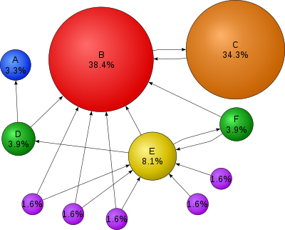
Source: Wikepedia
- $\mathbf{A} \in \{0,1\}^{n \times n}$ the connectivity matrix of webpages with entries
$n \approx 10^9$ in May 2017.
- $r_i = \sum_j a_{ij}$ is the out-degree of page $i$.
Larry Page imagined a random surfer wandering on internet according to following rules:
- From a page $i$ with $r_i>0$
- with probability $p$, (s)he randomly chooses a link $j$ from page $i$ (uniformly) and follows that link to the next page
- with probability $1-p$, (s)he randomly chooses one page from the set of all $n$ pages (uniformly) and proceeds to that page
- From a page $i$ with $r_i=0$ (a dangling page), (s)he randomly chooses one page from the set of all $n$ pages (uniformly) and proceeds to that page
- From a page $i$ with $r_i>0$
The process defines an $n$-state Markov chain, where each state corresponds to each page.
with interpretation $a_{ij}/r_i = 1/n$ if $r_i = 0$.
Stationary distribution of this Markov chain gives the score (long term probability of visit) of each page.
Stationary distribution can be obtained as the top left eigenvector of the transition matrix $\mathbf{P}=(p_{ij})$ corresponding to eigenvalue 1.
Equivalently it can be cast as a linear equation. $$ (\mathbf{I} - \mathbf{P}^T) \mathbf{x} = \mathbf{0}. $$
You've got to solve a linear equation with $10^9$ variables!
GE/LU will take $2 \times (10^9)^3/3/10^{12} \approx 6.66 \times 10^{14}$ seconds $\approx 20$ million years on a tera-flop supercomputer!
Iterative methods come to the rescue.
Splitting and fixed point iteration
- The key idea of iterative method for solving $\mathbf{A}\mathbf{x}=\mathbf{b}$ is to split the matrix $\mathbf{A}$ so that
where $\mathbf{M}$ is invertible and easy to invert.
- Then $\mathbf{A}\mathbf{x} = \mathbf{M}\mathbf{x} - \mathbf{K}\mathbf{x} = \mathbf{b}$ or
Thus a solution to $\mathbf{A}\mathbf{x}=\mathbf{b}$ is a fixed point of iteration $$ \mathbf{x}^{(t+1)} = \mathbf{M}^{-1}\mathbf{K}\mathbf{x}^{(t)} - \mathbf{M}^{-1}\mathbf{b} = \mathbf{R}\mathbf{x}^{(k)} - \mathbf{c} . $$
- Under a suitable choice of $\mathbf{R}$, i.e., splitting of $\mathbf{A}$, the sequence $\mathbf{x}^{(k)}$ generated by the above iteration converges to a solution $\mathbf{A}\mathbf{x}=\mathbf{b}$:
Let $\rho(\mathbf{R})=\max_{i=1,\dotsc,n}|\lambda_i(R)|$, where $\lambda_i(R)$ is the $i$th (complex) eigenvalue of $\mathbf{R}$. The iteration $\mathbf{x}^{(t+1)}=\mathbf{R}\mathbf{x}^{(t)} - \mathbf{c}$ converges to a solution to $\mathbf{A}\mathbf{x}=\mathbf{b}$ if and only if $\rho(\mathbf{R}) < 1$.
Jacobi's method
$$ x_i^{(t+1)} = \frac{b_i - \sum_{j=1}^{i-1} a_{ij} x_j^{(t)} - \sum_{j=i+1}^n a_{ij} x_j^{(t)}}{a_{ii}}. $$Split $\mathbf{A} = \mathbf{L} + \mathbf{D} + \mathbf{U}$ = (strictly lower triangular) + (diagonal) + (strictly upper triangular).
Take $\mathbf{M}=\mathbf{D}$ (easy to invert!) and $\mathbf{K}=-(\mathbf{L} + \mathbf{U})$:
i.e., $$ \mathbf{x}^{(t+1)} = - \mathbf{D}^{-1} (\mathbf{L} + \mathbf{U}) \mathbf{x}^{(t)} + \mathbf{D}^{-1} \mathbf{b} = - \mathbf{D}^{-1} \mathbf{A} \mathbf{x}^{(t)} + \mathbf{x}^{(t)} + \mathbf{D}^{-1} \mathbf{b}. $$
Convergence is guaranteed if $\mathbf{A}$ is striclty row diagonally dominant: $|a_{ii}| > \sum_{j\neq i}|a_{ij}|$.
One round costs $2n^2$ flops with an unstructured $\mathbf{A}$. Gain over GE/LU if converges in $o(n)$ iterations.
Saving is huge for sparse or structured $\mathbf{A}$. By structured, we mean the matrix-vector multiplication $\mathbf{A} \mathbf{v}$ is fast ($O(n)$ or $O(n \log n)$).
- Often the multiplication is implicit and $\mathbf{A}$ is not even stored, e.g., finite difference: $(\mathbf{A}\mathbf{v})_i = v_i - v_{i+1}$.
Gauss-Seidel method
$$ x_i^{(t+1)} = \frac{b_i - \sum_{j=1}^{i-1} a_{ij} x_j^{(t+1)} - \sum_{j=i+1}^n a_{ij} x_j^{(t)}}{a_{ii}}. $$Split $\mathbf{A} = \mathbf{L} + \mathbf{D} + \mathbf{U}$ = (strictly lower triangular) + (diagonal) + (strictly upper triangular) as Jacobi.
Take $\mathbf{M}=\mathbf{D}+\mathbf{L}$ (easy to invert, why?) and $\mathbf{K}=-\mathbf{U}$:
i.e., $$ \mathbf{x}^{(t+1)} = - (\mathbf{D} + \mathbf{L})^{-1} \mathbf{U} \mathbf{x}^{(t)} + (\mathbf{D} + \mathbf{L})^{-1} \mathbf{b}. $$
- Equivalent to
or $$ \mathbf{x}^{(t+1)} = \mathbf{D}^{-1}(- \mathbf{L} \mathbf{x}^{(t+1)} - \mathbf{U} \mathbf{x}^{(t)} + \mathbf{b}) $$ leading to the iteration.
"Coordinate descent" version of Jacobi.
Convergence is guaranteed if $\mathbf{A}$ is striclty row diagonally dominant.
Successive over-relaxation (SOR)
$$ x_i^{(t+1)} = \frac{\omega}{a_{ii}} \left( b_i - \sum_{j=1}^{i-1} a_{ij} x_j^{(t+1)} - \sum_{j=i+1}^n a_{ij} x_j^{(t)} \right)+ (1-\omega) x_i^{(t)}, $$$\omega=1$: Gauss-Seidel; $\omega \in (0, 1)$: underrelaxation; $\omega > 1$: overrelaxation
- Relaxation in hope of faster convergence
Split $\mathbf{A} = \mathbf{L} + \mathbf{D} + \mathbf{U}$ = (strictly lower triangular) + (diagonal) + (strictly upper triangular) as before.
Take $\mathbf{M}=\frac{1}{\omega}\mathbf{D}+\mathbf{L}$ (easy to invert, why?) and $\mathbf{K}=\frac{1-\omega}{\omega}\mathbf{D}-\mathbf{U}$:
Conjugate gradient method
Conjugate gradient and its variants are the top-notch iterative methods for solving huge, structured linear systems.
Key idea: solving $\mathbf{A} \mathbf{x} = \mathbf{b}$ is equivalent to minimizing the quadratic function $\frac{1}{2} \mathbf{x}^T \mathbf{A} \mathbf{x} - \mathbf{b}^T \mathbf{x}$ if $\mathbf{A}$ is positive definite.
Application to a fusion problem in physics:
| Method | Number of Iterations |
|---|---|
| Gauss Seidel | 208,000 |
| Block SOR methods | 765 |
| Incomplete Cholesky conjugate gradient | 25 |
- More on CG later.
MatrixDepot.jl
MatrixDepot.jl is an extensive collection of test matrices in Julia. After installation, we can check available test matrices by
using MatrixDepot

mdinfo()
include group.jl for user defined matrix generators
verify download of index files...
reading database
adding metadata...
adding svd data...
writing database
used remote sites are sparse.tamu.edu with MAT index and math.nist.gov with HTML index
Currently loaded Matrices
| builtin(#) | ||||
|---|---|---|---|---|
| 1 baart | 13 fiedler | 25 invhilb | 37 parter | 49 shaw |
| 2 binomial | 14 forsythe | 26 invol | 38 pascal | 50 smallworld |
| 3 blur | 15 foxgood | 27 kahan | 39 pei | 51 spikes |
| 4 cauchy | 16 frank | 28 kms | 40 phillips | 52 toeplitz |
| 5 chebspec | 17 gilbert | 29 lehmer | 41 poisson | 53 tridiag |
| 6 chow | 18 golub | 30 lotkin | 42 prolate | 54 triw |
| 7 circul | 19 gravity | 31 magic | 43 randcorr | 55 ursell |
| 8 clement | 20 grcar | 32 minij | 44 rando | 56 vand |
| 9 companion | 21 hadamard | 33 moler | 45 randsvd | 57 wathen |
| 10 deriv2 | 22 hankel | 34 neumann | 46 rohess | 58 wilkinson |
| 11 dingdong | 23 heat | 35 oscillate | 47 rosser | 59 wing |
| 12 erdrey | 24 hilb | 36 parallax | 48 sampling |
| user(#) |
|---|
| Groups | |||||||||||
|---|---|---|---|---|---|---|---|---|---|---|---|
| all | local | eigen | illcond | posdef | regprob | symmetric | |||||
| builtin | user | graph | inverse | random | sparse |
| Suite Sparse | of |
|---|---|
| 1 | 2893 |
| MatrixMarket | of |
|---|---|
| 0 | 498 |
# List matrices that are positive definite and sparse:
mdlist(:symmetric & :posdef & :sparse)
2-element Vector{String}:
 "poisson"
 "wathen"
# Get help on Poisson matrix
mdinfo("poisson")
Poisson Matrix (poisson)
A block tridiagonal matrix from Poisson’s equation. This matrix is sparse, symmetric positive definite and has known eigenvalues. The result is of type SparseMatrixCSC.
Input options:
- [type,] dim: the dimension of the matirx is
dim^2.
Groups: ["inverse", "symmetric", "posdef", "eigen", "sparse"]
References:
G. H. Golub and C. F. Van Loan, Matrix Computations, second edition, Johns Hopkins University Press, Baltimore, Maryland, 1989 (Section 4.5.4).
# Generate a Poisson matrix of dimension n=10
A = matrixdepot("poisson", 10)
100×100 SparseArrays.SparseMatrixCSC{Float64, Int64} with 460 stored entries:
⠻⣦⡀⠀⠑⢄⠀⠀⠀⠀⠀⠀⠀⠀⠀⠀⠀⠀⠀⠀⠀⠀⠀⠀⠀⠀⠀⠀⠀⠀⠀⠀⠀⠀⠀⠀⠀⠀⠀⠀
⠀⠈⠻⣦⠀⠀⠑⢄⠀⠀⠀⠀⠀⠀⠀⠀⠀⠀⠀⠀⠀⠀⠀⠀⠀⠀⠀⠀⠀⠀⠀⠀⠀⠀⠀⠀⠀⠀⠀⠀
⠑⢄⠀⠀⠻⣦⡀⠀⠑⢄⠀⠀⠀⠀⠀⠀⠀⠀⠀⠀⠀⠀⠀⠀⠀⠀⠀⠀⠀⠀⠀⠀⠀⠀⠀⠀⠀⠀⠀⠀
⠀⠀⠑⢄⠀⠈⠻⣦⠀⠀⠑⢄⠀⠀⠀⠀⠀⠀⠀⠀⠀⠀⠀⠀⠀⠀⠀⠀⠀⠀⠀⠀⠀⠀⠀⠀⠀⠀⠀⠀
⠀⠀⠀⠀⠑⢄⠀⠀⠻⣦⡀⠀⠑⢄⠀⠀⠀⠀⠀⠀⠀⠀⠀⠀⠀⠀⠀⠀⠀⠀⠀⠀⠀⠀⠀⠀⠀⠀⠀⠀
⠀⠀⠀⠀⠀⠀⠑⢄⠀⠈⠻⣦⠀⠀⠑⢄⠀⠀⠀⠀⠀⠀⠀⠀⠀⠀⠀⠀⠀⠀⠀⠀⠀⠀⠀⠀⠀⠀⠀⠀
⠀⠀⠀⠀⠀⠀⠀⠀⠑⢄⠀⠀⠻⣦⡀⠀⠑⢄⠀⠀⠀⠀⠀⠀⠀⠀⠀⠀⠀⠀⠀⠀⠀⠀⠀⠀⠀⠀⠀⠀
⠀⠀⠀⠀⠀⠀⠀⠀⠀⠀⠑⢄⠀⠈⠻⣦⠀⠀⠑⢄⠀⠀⠀⠀⠀⠀⠀⠀⠀⠀⠀⠀⠀⠀⠀⠀⠀⠀⠀⠀
⠀⠀⠀⠀⠀⠀⠀⠀⠀⠀⠀⠀⠑⢄⠀⠀⠻⣦⡀⠀⠱⢄⠀⠀⠀⠀⠀⠀⠀⠀⠀⠀⠀⠀⠀⠀⠀⠀⠀⠀
⠀⠀⠀⠀⠀⠀⠀⠀⠀⠀⠀⠀⠀⠀⠑⢄⠀⠈⠻⣦⠀⠀⠱⢄⠀⠀⠀⠀⠀⠀⠀⠀⠀⠀⠀⠀⠀⠀⠀⠀
⠀⠀⠀⠀⠀⠀⠀⠀⠀⠀⠀⠀⠀⠀⠀⠀⠑⢆⠀⠀⠻⣦⡀⠀⠑⢄⠀⠀⠀⠀⠀⠀⠀⠀⠀⠀⠀⠀⠀⠀
⠀⠀⠀⠀⠀⠀⠀⠀⠀⠀⠀⠀⠀⠀⠀⠀⠀⠀⠑⢆⠀⠈⠻⣦⠀⠀⠑⢄⠀⠀⠀⠀⠀⠀⠀⠀⠀⠀⠀⠀
⠀⠀⠀⠀⠀⠀⠀⠀⠀⠀⠀⠀⠀⠀⠀⠀⠀⠀⠀⠀⠑⢄⠀⠀⠻⣦⡀⠀⠑⢄⠀⠀⠀⠀⠀⠀⠀⠀⠀⠀
⠀⠀⠀⠀⠀⠀⠀⠀⠀⠀⠀⠀⠀⠀⠀⠀⠀⠀⠀⠀⠀⠀⠑⢄⠀⠈⠻⣦⠀⠀⠑⢄⠀⠀⠀⠀⠀⠀⠀⠀
⠀⠀⠀⠀⠀⠀⠀⠀⠀⠀⠀⠀⠀⠀⠀⠀⠀⠀⠀⠀⠀⠀⠀⠀⠑⢄⠀⠀⠻⣦⡀⠀⠑⢄⠀⠀⠀⠀⠀⠀
⠀⠀⠀⠀⠀⠀⠀⠀⠀⠀⠀⠀⠀⠀⠀⠀⠀⠀⠀⠀⠀⠀⠀⠀⠀⠀⠑⢄⠀⠈⠻⣦⠀⠀⠑⢄⠀⠀⠀⠀
⠀⠀⠀⠀⠀⠀⠀⠀⠀⠀⠀⠀⠀⠀⠀⠀⠀⠀⠀⠀⠀⠀⠀⠀⠀⠀⠀⠀⠑⢄⠀⠀⠻⣦⡀⠀⠑⢄⠀⠀
⠀⠀⠀⠀⠀⠀⠀⠀⠀⠀⠀⠀⠀⠀⠀⠀⠀⠀⠀⠀⠀⠀⠀⠀⠀⠀⠀⠀⠀⠀⠑⢄⠀⠈⠻⣦⠀⠀⠑⢄
⠀⠀⠀⠀⠀⠀⠀⠀⠀⠀⠀⠀⠀⠀⠀⠀⠀⠀⠀⠀⠀⠀⠀⠀⠀⠀⠀⠀⠀⠀⠀⠀⠑⢄⠀⠀⠻⣦⡀⠀
⠀⠀⠀⠀⠀⠀⠀⠀⠀⠀⠀⠀⠀⠀⠀⠀⠀⠀⠀⠀⠀⠀⠀⠀⠀⠀⠀⠀⠀⠀⠀⠀⠀⠀⠑⢄⠀⠈⠻⣦
using UnicodePlots
spy(A)
       ⠀⠀⠀⠀⠀⠀⠀⠀⠀⠀⠀⠀⠀⠀Sparsity Pattern⠀⠀⠀⠀⠀⠀⠀⠀⠀⠀⠀⠀⠀⠀
       ┌──────────────────────────────────────────┐
     1 │⠻⣦⡀⠀⠘⢄⠀⠀⠀⠀⠀⠀⠀⠀⠀⠀⠀⠀⠀⠀⠀⠀⠀⠀⠀⠀⠀⠀⠀⠀⠀⠀⠀⠀⠀⠀⠀⠀⠀⠀⠀⠀│ > 0
       │⠀⠈⠻⣦⡀⠀⠉⢆⠀⠀⠀⠀⠀⠀⠀⠀⠀⠀⠀⠀⠀⠀⠀⠀⠀⠀⠀⠀⠀⠀⠀⠀⠀⠀⠀⠀⠀⠀⠀⠀⠀⠀│ < 0
       │⠒⢄⠀⠈⠱⣦⡀⠀⠑⢢⠀⠀⠀⠀⠀⠀⠀⠀⠀⠀⠀⠀⠀⠀⠀⠀⠀⠀⠀⠀⠀⠀⠀⠀⠀⠀⠀⠀⠀⠀⠀⠀│
       │⠀⠀⠣⢄⠀⠈⠻⣦⡀⠀⠑⠤⡀⠀⠀⠀⠀⠀⠀⠀⠀⠀⠀⠀⠀⠀⠀⠀⠀⠀⠀⠀⠀⠀⠀⠀⠀⠀⠀⠀⠀⠀│
       │⠀⠀⠀⠀⠱⣀⠀⠈⠱⣦⡀⠀⠑⢄⡀⠀⠀⠀⠀⠀⠀⠀⠀⠀⠀⠀⠀⠀⠀⠀⠀⠀⠀⠀⠀⠀⠀⠀⠀⠀⠀⠀│
       │⠀⠀⠀⠀⠀⠀⠑⡄⠀⠈⠻⣦⡀⠀⠘⢄⠀⠀⠀⠀⠀⠀⠀⠀⠀⠀⠀⠀⠀⠀⠀⠀⠀⠀⠀⠀⠀⠀⠀⠀⠀⠀│
       │⠀⠀⠀⠀⠀⠀⠀⠈⠑⢄⠀⠈⠱⣦⡀⠀⠉⢆⠀⠀⠀⠀⠀⠀⠀⠀⠀⠀⠀⠀⠀⠀⠀⠀⠀⠀⠀⠀⠀⠀⠀⠀│
       │⠀⠀⠀⠀⠀⠀⠀⠀⠀⠈⠒⢄⠀⠈⠻⣦⡀⠀⠑⢢⠀⠀⠀⠀⠀⠀⠀⠀⠀⠀⠀⠀⠀⠀⠀⠀⠀⠀⠀⠀⠀⠀│
       │⠀⠀⠀⠀⠀⠀⠀⠀⠀⠀⠀⠀⠣⢄⠀⠈⠛⣤⡀⠀⠑⠤⡀⠀⠀⠀⠀⠀⠀⠀⠀⠀⠀⠀⠀⠀⠀⠀⠀⠀⠀⠀│
       │⠀⠀⠀⠀⠀⠀⠀⠀⠀⠀⠀⠀⠀⠀⠱⣀⠀⠈⠻⣦⡀⠀⠑⢄⡀⠀⠀⠀⠀⠀⠀⠀⠀⠀⠀⠀⠀⠀⠀⠀⠀⠀│
       │⠀⠀⠀⠀⠀⠀⠀⠀⠀⠀⠀⠀⠀⠀⠀⠀⠑⡄⠀⠈⠛⣤⡀⠀⠘⢄⠀⠀⠀⠀⠀⠀⠀⠀⠀⠀⠀⠀⠀⠀⠀⠀│
       │⠀⠀⠀⠀⠀⠀⠀⠀⠀⠀⠀⠀⠀⠀⠀⠀⠀⠈⠑⢄⠀⠈⠻⣦⡀⠀⠉⢆⠀⠀⠀⠀⠀⠀⠀⠀⠀⠀⠀⠀⠀⠀│
       │⠀⠀⠀⠀⠀⠀⠀⠀⠀⠀⠀⠀⠀⠀⠀⠀⠀⠀⠀⠈⠒⢄⠀⠈⠛⣤⡀⠀⠑⢢⠀⠀⠀⠀⠀⠀⠀⠀⠀⠀⠀⠀│
       │⠀⠀⠀⠀⠀⠀⠀⠀⠀⠀⠀⠀⠀⠀⠀⠀⠀⠀⠀⠀⠀⠀⠣⢄⠀⠈⠻⣦⡀⠀⠑⠤⡀⠀⠀⠀⠀⠀⠀⠀⠀⠀│
       │⠀⠀⠀⠀⠀⠀⠀⠀⠀⠀⠀⠀⠀⠀⠀⠀⠀⠀⠀⠀⠀⠀⠀⠀⠱⣀⠀⠈⠻⢆⡀⠀⠑⢄⡀⠀⠀⠀⠀⠀⠀⠀│
       │⠀⠀⠀⠀⠀⠀⠀⠀⠀⠀⠀⠀⠀⠀⠀⠀⠀⠀⠀⠀⠀⠀⠀⠀⠀⠀⠑⡄⠀⠈⠻⣦⡀⠀⠘⢄⠀⠀⠀⠀⠀⠀│
       │⠀⠀⠀⠀⠀⠀⠀⠀⠀⠀⠀⠀⠀⠀⠀⠀⠀⠀⠀⠀⠀⠀⠀⠀⠀⠀⠀⠈⠑⢄⠀⠈⠻⢆⡀⠀⠉⢆⠀⠀⠀⠀│
       │⠀⠀⠀⠀⠀⠀⠀⠀⠀⠀⠀⠀⠀⠀⠀⠀⠀⠀⠀⠀⠀⠀⠀⠀⠀⠀⠀⠀⠀⠈⠒⢄⠀⠈⠻⣦⡀⠀⠑⢢⠀⠀│
       │⠀⠀⠀⠀⠀⠀⠀⠀⠀⠀⠀⠀⠀⠀⠀⠀⠀⠀⠀⠀⠀⠀⠀⠀⠀⠀⠀⠀⠀⠀⠀⠀⠣⢄⠀⠈⠻⢆⡀⠀⠑⠤│
       │⠀⠀⠀⠀⠀⠀⠀⠀⠀⠀⠀⠀⠀⠀⠀⠀⠀⠀⠀⠀⠀⠀⠀⠀⠀⠀⠀⠀⠀⠀⠀⠀⠀⠀⠱⣀⠀⠈⠻⣦⡀⠀│
   100 │⠀⠀⠀⠀⠀⠀⠀⠀⠀⠀⠀⠀⠀⠀⠀⠀⠀⠀⠀⠀⠀⠀⠀⠀⠀⠀⠀⠀⠀⠀⠀⠀⠀⠀⠀⠀⠑⡄⠀⠈⠻⣦│
       └──────────────────────────────────────────┘
       ⠀1⠀⠀⠀⠀⠀⠀⠀⠀⠀⠀⠀⠀⠀⠀⠀⠀⠀⠀⠀⠀⠀⠀⠀⠀⠀⠀⠀⠀⠀⠀⠀⠀⠀⠀⠀⠀⠀⠀100⠀
       ⠀⠀⠀⠀⠀⠀⠀⠀⠀⠀⠀⠀⠀⠀⠀⠀⠀⠀nz = 460⠀⠀⠀⠀⠀⠀⠀⠀⠀⠀⠀⠀⠀⠀⠀⠀⠀⠀
# Get help on Wathen matrix
mdinfo("wathen")
Wathen Matrix (wathen)
Wathen Matrix is a sparse, symmetric positive, random matrix arose from the finite element method. The generated matrix is the consistent mass matrix for a regular nx-by-ny grid of 8-nodes.
Input options:
- [type,] nx, ny: the dimension of the matrix is equal to
3 * nx * ny + 2 * nx * ny + 1. - [type,] n:
nx = ny = n.
Groups: ["symmetric", "posdef", "eigen", "random", "sparse"]
References:
A. J. Wathen, Realistic eigenvalue bounds for the Galerkin mass matrix, IMA J. Numer. Anal., 7 (1987), pp. 449-457.
# Generate a Wathen matrix of dimension n=5
A = matrixdepot("wathen", 5)
96×96 SparseArrays.SparseMatrixCSC{Float64, Int64} with 1256 stored entries:
⠿⣧⣀⠀⠸⣧⡀⠿⣧⣀⠀⠀⠀⠀⠀⠀⠀⠀⠀⠀⠀⠀⠀⠀⠀⠀⠀⠀⠀⠀⠀⠀⠀⠀⠀⠀⠀⠀⠀⠀
⠀⠘⢻⣶⡀⠘⣇⠀⠘⢻⣶⡀⠀⠀⠀⠀⠀⠀⠀⠀⠀⠀⠀⠀⠀⠀⠀⠀⠀⠀⠀⠀⠀⠀⠀⠀⠀⠀⠀⠀
⠶⣦⣀⠈⠱⣦⡉⠶⣦⣀⠈⠁⠀⠀⠀⠀⠀⠀⠀⠀⠀⠀⠀⠀⠀⠀⠀⠀⠀⠀⠀⠀⠀⠀⠀⠀⠀⠀⠀⠀
⣤⡌⠉⠙⢣⡌⠛⣤⡌⠉⠙⢣⡄⠀⣤⡄⠀⠀⠀⠀⠀⠀⠀⠀⠀⠀⠀⠀⠀⠀⠀⠀⠀⠀⠀⠀⠀⠀⠀⠀
⠉⢻⣶⣀⠈⢻⡆⠉⢻⣶⣀⠈⢻⣆⠉⠛⣷⣀⠀⠀⠀⠀⠀⠀⠀⠀⠀⠀⠀⠀⠀⠀⠀⠀⠀⠀⠀⠀⠀⠀
⠀⠀⠘⠻⠆⠀⠷⣀⡀⠘⠻⢆⡀⠻⣀⡀⠘⠻⠶⠀⠀⠀⠀⠀⠀⠀⠀⠀⠀⠀⠀⠀⠀⠀⠀⠀⠀⠀⠀⠀
⠀⠀⠀⠀⠀⠀⠀⠉⠻⢶⣤⡈⠻⣦⠉⠛⢷⣤⣀⠀⠀⠀⠀⠀⠀⠀⠀⠀⠀⠀⠀⠀⠀⠀⠀⠀⠀⠀⠀⠀
⠀⠀⠀⠀⠀⠀⠀⠿⣧⠀⠀⠸⣧⠀⠿⣧⡄⠀⠸⣧⠀⠿⣧⡄⠀⠀⠀⠀⠀⠀⠀⠀⠀⠀⠀⠀⠀⠀⠀⠀
⠀⠀⠀⠀⠀⠀⠀⠀⠙⢻⣶⡀⠙⣷⠀⠉⢻⣶⣀⠙⣷⡀⠉⢻⣶⣀⠀⠀⠀⠀⠀⠀⠀⠀⠀⠀⠀⠀⠀⠀
⠀⠀⠀⠀⠀⠀⠀⠀⠀⠀⠘⠃⠀⠘⠶⣦⣄⠘⠻⣦⡘⠷⣦⣄⠘⠛⠀⠀⠀⠀⠀⠀⠀⠀⠀⠀⠀⠀⠀⠀
⠀⠀⠀⠀⠀⠀⠀⠀⠀⠀⠀⠀⠀⠀⣤⡄⠙⠻⢶⡌⠻⣦⡄⠙⠻⠶⡄⠀⢠⡄⠀⠀⠀⠀⠀⠀⠀⠀⠀⠀
⠀⠀⠀⠀⠀⠀⠀⠀⠀⠀⠀⠀⠀⠀⠉⠿⣧⣀⠈⢿⣄⠉⠿⣧⣀⠀⢿⣄⠈⠿⣧⣄⠀⠀⠀⠀⠀⠀⠀⠀
⠀⠀⠀⠀⠀⠀⠀⠀⠀⠀⠀⠀⠀⠀⠀⠀⠘⢻⣶⠀⢻⡆⠀⠘⢻⣶⠀⢻⡆⠀⠀⢻⣶⠀⠀⠀⠀⠀⠀⠀
⠀⠀⠀⠀⠀⠀⠀⠀⠀⠀⠀⠀⠀⠀⠀⠀⠀⠀⠀⠀⠀⠉⠛⢷⣤⣀⠻⣦⡈⠛⠷⣦⣀⠀⠀⠀⠀⠀⠀⠀
⠀⠀⠀⠀⠀⠀⠀⠀⠀⠀⠀⠀⠀⠀⠀⠀⠀⠀⠀⠀⠀⠶⣦⡄⠈⠉⣦⠈⠱⣦⡄⠈⠉⢶⠀⠰⣦⡄⠀⠀
⠀⠀⠀⠀⠀⠀⠀⠀⠀⠀⠀⠀⠀⠀⠀⠀⠀⠀⠀⠀⠀⠀⠉⢿⣤⣀⠹⣧⡀⠉⠿⣧⣀⠸⣧⡀⠉⠿⣧⣀
⠀⠀⠀⠀⠀⠀⠀⠀⠀⠀⠀⠀⠀⠀⠀⠀⠀⠀⠀⠀⠀⠀⠀⠀⠘⠛⠀⠘⢣⣄⣀⡘⠛⣤⡘⢣⣄⣀⡘⠛
⠀⠀⠀⠀⠀⠀⠀⠀⠀⠀⠀⠀⠀⠀⠀⠀⠀⠀⠀⠀⠀⠀⠀⠀⠀⠀⠀⠀⢀⡀⠉⠻⠶⣈⠻⢆⡀⠉⠻⠶
⠀⠀⠀⠀⠀⠀⠀⠀⠀⠀⠀⠀⠀⠀⠀⠀⠀⠀⠀⠀⠀⠀⠀⠀⠀⠀⠀⠀⠈⠿⣧⡄⠀⢹⡄⠈⠿⣧⡄⠀
⠀⠀⠀⠀⠀⠀⠀⠀⠀⠀⠀⠀⠀⠀⠀⠀⠀⠀⠀⠀⠀⠀⠀⠀⠀⠀⠀⠀⠀⠀⠉⢻⣶⠈⢻⡆⠀⠉⢻⣶
spy(A)
      ⠀⠀⠀⠀⠀⠀⠀⠀⠀⠀⠀⠀⠀⠀Sparsity Pattern⠀⠀⠀⠀⠀⠀⠀⠀⠀⠀⠀⠀⠀⠀
      ┌──────────────────────────────────────────┐
    1 │⠿⣧⡄⠀⠀⢿⡄⠸⢿⣤⠀⠀⠀⠀⠀⠀⠀⠀⠀⠀⠀⠀⠀⠀⠀⠀⠀⠀⠀⠀⠀⠀⠀⠀⠀⠀⠀⠀⠀⠀⠀⠀│ > 0
      │⠀⠉⠿⣧⣀⠈⣧⡀⠈⠹⣧⣄⡀⠀⠀⠀⠀⠀⠀⠀⠀⠀⠀⠀⠀⠀⠀⠀⠀⠀⠀⠀⠀⠀⠀⠀⠀⠀⠀⠀⠀⠀│ < 0
      │⣤⣄⡀⠘⠛⣤⡘⢣⣤⣀⠀⠛⠃⠀⠀⠀⠀⠀⠀⠀⠀⠀⠀⠀⠀⠀⠀⠀⠀⠀⠀⠀⠀⠀⠀⠀⠀⠀⠀⠀⠀⠀│
      │⣀⡉⠉⠻⠶⣈⠻⢆⣈⠉⠛⠷⢆⠀⠀⣀⡀⠀⠀⠀⠀⠀⠀⠀⠀⠀⠀⠀⠀⠀⠀⠀⠀⠀⠀⠀⠀⠀⠀⠀⠀⠀│
      │⠛⣷⣆⡀⠀⢻⡆⠘⢻⣶⡀⠀⢸⣆⠀⠛⣷⣀⠀⠀⠀⠀⠀⠀⠀⠀⠀⠀⠀⠀⠀⠀⠀⠀⠀⠀⠀⠀⠀⠀⠀⠀│
      │⠀⠀⠉⢿⣤⠀⢿⡄⠀⠈⠿⣧⡄⠹⣧⠀⠈⠹⢿⡄⠀⠀⠀⠀⠀⠀⠀⠀⠀⠀⠀⠀⠀⠀⠀⠀⠀⠀⠀⠀⠀⠀│
      │⠀⠀⠀⠈⠉⠀⠈⠑⠲⢶⣄⡉⠱⣦⡉⠒⢶⣤⣈⠁⠀⠀⠀⠀⠀⠀⠀⠀⠀⠀⠀⠀⠀⠀⠀⠀⠀⠀⠀⠀⠀⠀│
      │⠀⠀⠀⠀⠀⠀⠀⢠⣤⠀⠉⠛⢣⠈⠛⣤⡄⠈⠙⢣⡄⠀⢠⡄⠀⠀⠀⠀⠀⠀⠀⠀⠀⠀⠀⠀⠀⠀⠀⠀⠀⠀│
      │⠀⠀⠀⠀⠀⠀⠀⠈⠙⢻⣆⡀⠘⣷⡀⠉⢻⣶⣀⠈⢻⣆⠈⠛⣷⣆⠀⠀⠀⠀⠀⠀⠀⠀⠀⠀⠀⠀⠀⠀⠀⠀│
      │⠀⠀⠀⠀⠀⠀⠀⠀⠀⠀⠛⠷⠆⠘⠷⣀⡀⠘⠻⢆⡀⠻⢆⡀⠀⠻⠶⠀⠀⠀⠀⠀⠀⠀⠀⠀⠀⠀⠀⠀⠀⠀│
      │⠀⠀⠀⠀⠀⠀⠀⠀⠀⠀⠀⠀⠀⠀⠀⠉⠻⢶⣤⡈⠻⣦⡈⠛⠷⣦⣀⠀⠀⠀⠀⠀⠀⠀⠀⠀⠀⠀⠀⠀⠀⠀│
      │⠀⠀⠀⠀⠀⠀⠀⠀⠀⠀⠀⠀⠀⠀⠀⠶⣦⠀⠈⠱⣦⠈⠱⣦⡄⠈⠉⢶⡄⠰⢶⣤⠀⠀⠀⠀⠀⠀⠀⠀⠀⠀│
      │⠀⠀⠀⠀⠀⠀⠀⠀⠀⠀⠀⠀⠀⠀⠀⠀⠹⢿⣤⡀⠹⣧⡀⠉⠿⣧⣀⠈⢿⡄⠈⠹⣧⣄⡀⠀⠀⠀⠀⠀⠀⠀│
      │⠀⠀⠀⠀⠀⠀⠀⠀⠀⠀⠀⠀⠀⠀⠀⠀⠀⠀⠘⠃⠀⠘⢣⣄⡀⠘⠛⣤⡀⢣⣤⣀⠀⠛⠃⠀⠀⠀⠀⠀⠀⠀│
      │⠀⠀⠀⠀⠀⠀⠀⠀⠀⠀⠀⠀⠀⠀⠀⠀⠀⠀⠀⠀⠀⠀⢀⡉⠛⠷⠤⣈⠻⢆⣈⠙⠷⠦⢄⡀⠀⣀⡀⠀⠀⠀│
      │⠀⠀⠀⠀⠀⠀⠀⠀⠀⠀⠀⠀⠀⠀⠀⠀⠀⠀⠀⠀⠀⠀⠘⣷⣆⡀⠀⢻⣆⠘⢻⣶⡀⠀⠘⣷⠀⠛⣷⣀⠀⠀│
      │⠀⠀⠀⠀⠀⠀⠀⠀⠀⠀⠀⠀⠀⠀⠀⠀⠀⠀⠀⠀⠀⠀⠀⠀⠉⢿⣤⠀⠹⡇⠀⠈⠿⣧⡄⠸⣧⠀⠈⠹⢿⣤│
      │⠀⠀⠀⠀⠀⠀⠀⠀⠀⠀⠀⠀⠀⠀⠀⠀⠀⠀⠀⠀⠀⠀⠀⠀⠀⠈⠉⠀⠀⠱⢶⣤⣀⡉⠱⣦⡉⠶⣦⣀⣈⠉│
      │⠀⠀⠀⠀⠀⠀⠀⠀⠀⠀⠀⠀⠀⠀⠀⠀⠀⠀⠀⠀⠀⠀⠀⠀⠀⠀⠀⠀⠀⢠⣤⠀⠉⠛⢣⡌⠛⣤⡄⠈⠙⠛│
      │⠀⠀⠀⠀⠀⠀⠀⠀⠀⠀⠀⠀⠀⠀⠀⠀⠀⠀⠀⠀⠀⠀⠀⠀⠀⠀⠀⠀⠀⠈⠙⢻⣆⡀⠈⢻⡀⠉⢻⣶⣀⠀│
   96 │⠀⠀⠀⠀⠀⠀⠀⠀⠀⠀⠀⠀⠀⠀⠀⠀⠀⠀⠀⠀⠀⠀⠀⠀⠀⠀⠀⠀⠀⠀⠀⠀⠛⣷⡆⠘⣷⠀⠀⠘⢻⣶│
      └──────────────────────────────────────────┘
      ⠀1⠀⠀⠀⠀⠀⠀⠀⠀⠀⠀⠀⠀⠀⠀⠀⠀⠀⠀⠀⠀⠀⠀⠀⠀⠀⠀⠀⠀⠀⠀⠀⠀⠀⠀⠀⠀⠀⠀⠀96⠀
      ⠀⠀⠀⠀⠀⠀⠀⠀⠀⠀⠀⠀⠀⠀⠀⠀⠀⠀nz = 1256⠀⠀⠀⠀⠀⠀⠀⠀⠀⠀⠀⠀⠀⠀⠀⠀⠀
Numerical examples
The IterativeSolvers.jl package implements most commonly used iterative solvers.
Generate test matrix
using BenchmarkTools, IterativeSolvers, LinearAlgebra, MatrixDepot, Random

Random.seed!(280)

n = 100
# Poisson matrix of dimension n^2=10000, pd and sparse
A = matrixdepot("poisson", n)
@show typeof(A)
# dense matrix representation of A
Afull = convert(Matrix, A)
@show typeof(Afull)
# sparsity level
count(!iszero, A) / length(A)
typeof(A) = SparseArrays.SparseMatrixCSC{Float64, Int64}
typeof(Afull) = Matrix{Float64}
0.000496
spy(A)
         ⠀⠀⠀⠀⠀⠀⠀⠀⠀⠀⠀⠀⠀⠀Sparsity Pattern⠀⠀⠀⠀⠀⠀⠀⠀⠀⠀⠀⠀⠀⠀
         ┌──────────────────────────────────────────┐
       1 │⠻⣦⡀⠀⠀⠀⠀⠀⠀⠀⠀⠀⠀⠀⠀⠀⠀⠀⠀⠀⠀⠀⠀⠀⠀⠀⠀⠀⠀⠀⠀⠀⠀⠀⠀⠀⠀⠀⠀⠀⠀⠀│ > 0
         │⠀⠈⠻⣦⡀⠀⠀⠀⠀⠀⠀⠀⠀⠀⠀⠀⠀⠀⠀⠀⠀⠀⠀⠀⠀⠀⠀⠀⠀⠀⠀⠀⠀⠀⠀⠀⠀⠀⠀⠀⠀⠀│ < 0
         │⠀⠀⠀⠈⠻⣦⡀⠀⠀⠀⠀⠀⠀⠀⠀⠀⠀⠀⠀⠀⠀⠀⠀⠀⠀⠀⠀⠀⠀⠀⠀⠀⠀⠀⠀⠀⠀⠀⠀⠀⠀⠀│
         │⠀⠀⠀⠀⠀⠈⠻⣦⡀⠀⠀⠀⠀⠀⠀⠀⠀⠀⠀⠀⠀⠀⠀⠀⠀⠀⠀⠀⠀⠀⠀⠀⠀⠀⠀⠀⠀⠀⠀⠀⠀⠀│
         │⠀⠀⠀⠀⠀⠀⠀⠈⠻⣦⡀⠀⠀⠀⠀⠀⠀⠀⠀⠀⠀⠀⠀⠀⠀⠀⠀⠀⠀⠀⠀⠀⠀⠀⠀⠀⠀⠀⠀⠀⠀⠀│
         │⠀⠀⠀⠀⠀⠀⠀⠀⠀⠈⠻⣦⡀⠀⠀⠀⠀⠀⠀⠀⠀⠀⠀⠀⠀⠀⠀⠀⠀⠀⠀⠀⠀⠀⠀⠀⠀⠀⠀⠀⠀⠀│
         │⠀⠀⠀⠀⠀⠀⠀⠀⠀⠀⠀⠈⠻⣦⡀⠀⠀⠀⠀⠀⠀⠀⠀⠀⠀⠀⠀⠀⠀⠀⠀⠀⠀⠀⠀⠀⠀⠀⠀⠀⠀⠀│
         │⠀⠀⠀⠀⠀⠀⠀⠀⠀⠀⠀⠀⠀⠈⠻⣦⡀⠀⠀⠀⠀⠀⠀⠀⠀⠀⠀⠀⠀⠀⠀⠀⠀⠀⠀⠀⠀⠀⠀⠀⠀⠀│
         │⠀⠀⠀⠀⠀⠀⠀⠀⠀⠀⠀⠀⠀⠀⠀⠈⠻⣦⡀⠀⠀⠀⠀⠀⠀⠀⠀⠀⠀⠀⠀⠀⠀⠀⠀⠀⠀⠀⠀⠀⠀⠀│
         │⠀⠀⠀⠀⠀⠀⠀⠀⠀⠀⠀⠀⠀⠀⠀⠀⠀⠈⠻⣦⡀⠀⠀⠀⠀⠀⠀⠀⠀⠀⠀⠀⠀⠀⠀⠀⠀⠀⠀⠀⠀⠀│
         │⠀⠀⠀⠀⠀⠀⠀⠀⠀⠀⠀⠀⠀⠀⠀⠀⠀⠀⠀⠈⠻⣦⡀⠀⠀⠀⠀⠀⠀⠀⠀⠀⠀⠀⠀⠀⠀⠀⠀⠀⠀⠀│
         │⠀⠀⠀⠀⠀⠀⠀⠀⠀⠀⠀⠀⠀⠀⠀⠀⠀⠀⠀⠀⠀⠈⠻⣦⡀⠀⠀⠀⠀⠀⠀⠀⠀⠀⠀⠀⠀⠀⠀⠀⠀⠀│
         │⠀⠀⠀⠀⠀⠀⠀⠀⠀⠀⠀⠀⠀⠀⠀⠀⠀⠀⠀⠀⠀⠀⠀⠈⠻⣦⡀⠀⠀⠀⠀⠀⠀⠀⠀⠀⠀⠀⠀⠀⠀⠀│
         │⠀⠀⠀⠀⠀⠀⠀⠀⠀⠀⠀⠀⠀⠀⠀⠀⠀⠀⠀⠀⠀⠀⠀⠀⠀⠈⠻⣦⡀⠀⠀⠀⠀⠀⠀⠀⠀⠀⠀⠀⠀⠀│
         │⠀⠀⠀⠀⠀⠀⠀⠀⠀⠀⠀⠀⠀⠀⠀⠀⠀⠀⠀⠀⠀⠀⠀⠀⠀⠀⠀⠈⠻⣦⡀⠀⠀⠀⠀⠀⠀⠀⠀⠀⠀⠀│
         │⠀⠀⠀⠀⠀⠀⠀⠀⠀⠀⠀⠀⠀⠀⠀⠀⠀⠀⠀⠀⠀⠀⠀⠀⠀⠀⠀⠀⠀⠈⠻⣦⡀⠀⠀⠀⠀⠀⠀⠀⠀⠀│
         │⠀⠀⠀⠀⠀⠀⠀⠀⠀⠀⠀⠀⠀⠀⠀⠀⠀⠀⠀⠀⠀⠀⠀⠀⠀⠀⠀⠀⠀⠀⠀⠈⠻⣦⡀⠀⠀⠀⠀⠀⠀⠀│
         │⠀⠀⠀⠀⠀⠀⠀⠀⠀⠀⠀⠀⠀⠀⠀⠀⠀⠀⠀⠀⠀⠀⠀⠀⠀⠀⠀⠀⠀⠀⠀⠀⠀⠈⠻⣦⡀⠀⠀⠀⠀⠀│
         │⠀⠀⠀⠀⠀⠀⠀⠀⠀⠀⠀⠀⠀⠀⠀⠀⠀⠀⠀⠀⠀⠀⠀⠀⠀⠀⠀⠀⠀⠀⠀⠀⠀⠀⠀⠈⠻⣦⡀⠀⠀⠀│
         │⠀⠀⠀⠀⠀⠀⠀⠀⠀⠀⠀⠀⠀⠀⠀⠀⠀⠀⠀⠀⠀⠀⠀⠀⠀⠀⠀⠀⠀⠀⠀⠀⠀⠀⠀⠀⠀⠈⠻⣦⡀⠀│
   10000 │⠀⠀⠀⠀⠀⠀⠀⠀⠀⠀⠀⠀⠀⠀⠀⠀⠀⠀⠀⠀⠀⠀⠀⠀⠀⠀⠀⠀⠀⠀⠀⠀⠀⠀⠀⠀⠀⠀⠀⠈⠻⣦│
         └──────────────────────────────────────────┘
         ⠀1⠀⠀⠀⠀⠀⠀⠀⠀⠀⠀⠀⠀⠀⠀⠀⠀⠀⠀⠀⠀⠀⠀⠀⠀⠀⠀⠀⠀⠀⠀⠀⠀⠀⠀⠀⠀10000⠀
         ⠀⠀⠀⠀⠀⠀⠀⠀⠀⠀⠀⠀⠀⠀⠀⠀⠀nz = 49600⠀⠀⠀⠀⠀⠀⠀⠀⠀⠀⠀⠀⠀⠀⠀⠀⠀
# storage difference
Base.summarysize(A), Base.summarysize(Afull)
(873768, 800000040)
Matrix-vector muliplication
# randomly generated vector of length n^2
b = randn(n^2)
# dense matrix-vector multiplication
@benchmark $Afull * $b
BenchmarkTools.Trial: 116 samples with 1 evaluation.
 Range (min … max):  41.223 ms …  45.530 ms  ┊ GC (min … max): 0.00% … 0.00%
 Time  (median):     43.316 ms               ┊ GC (median):    0.00%
 Time  (mean ± σ):   43.407 ms ± 846.034 μs  ┊ GC (mean ± σ):  0.00% ± 0.00%

                   ▂▄ ▂▄█▄▂     ▄       ▆█▄▂▆  ▂    ▂
  ▄▁▄▁▁▁▁▄▁▁▁▁▄▄▄▄▄█████████▄▆▆▄█▄▄▄▄▁▆▆██████▄█▁▄▆▄██▁▁▁▁▁▁▁▄ ▄
  41.2 ms         Histogram: frequency by time         45.3 ms <

 Memory estimate: 78.20 KiB, allocs estimate: 2.
# sparse matrix-vector multiplication
@benchmark $A * $b
BenchmarkTools.Trial: 10000 samples with 1 evaluation.
 Range (min … max):  63.610 μs …  44.016 ms  ┊ GC (min … max): 0.00% … 99.70%
 Time  (median):     85.806 μs               ┊ GC (median):    0.00%
 Time  (mean ± σ):   94.585 μs ± 439.588 μs  ┊ GC (mean ± σ):  4.64% ±  1.00%

          ▄▇██▇▆▆▅▄▃▂▂ ▁                                       ▂
  ▆▅▆▄▃▁▄▅████████████████▇▆▆▇▇███▇█▇▅▇▇▇▇▇▇▆▆▆▆▇▇▇▇▆▇▆▆▅▆▇▇▆▇ █
  63.6 μs       Histogram: log(frequency) by time       179 μs <

 Memory estimate: 78.20 KiB, allocs estimate: 2.
Dense solve via Cholesky
# record the Cholesky solution
xchol = cholesky(Afull) \ b;
# dense solve via Cholesky
@benchmark cholesky($Afull) \ $b
BenchmarkTools.Trial: 2 samples with 1 evaluation.
 Range (min … max):  2.933 s …    3.085 s  ┊ GC (min … max): 0.02% … 1.46%
 Time  (median):     3.009 s               ┊ GC (median):    0.76%
 Time  (mean ± σ):   3.009 s ± 107.518 ms  ┊ GC (mean ± σ):  0.76% ± 1.02%

  █                                                        █
  █▁▁▁▁▁▁▁▁▁▁▁▁▁▁▁▁▁▁▁▁▁▁▁▁▁▁▁▁▁▁▁▁▁▁▁▁▁▁▁▁▁▁▁▁▁▁▁▁▁▁▁▁▁▁▁▁█ ▁
  2.93 s         Histogram: frequency by time         3.09 s <

 Memory estimate: 763.02 MiB, allocs estimate: 6.
Jacobi solver
It seems that Jacobi solver doesn't give the correct answer.
xjacobi = jacobi(A, b)
@show norm(xjacobi - xchol)
norm(xjacobi - xchol) = 553.3696146722076
553.3696146722076
Documentation reveals that the default value of maxiter is 10. A couple trial runs shows that 30000 Jacobi iterations are enough to get an accurate solution.
xjacobi = jacobi(A, b, maxiter=30000)
@show norm(xjacobi - xchol)
norm(xjacobi - xchol) = 0.0001726309300532125
0.0001726309300532125
@benchmark jacobi($A, $b, maxiter=30000)
BenchmarkTools.Trial: 3 samples with 1 evaluation.
 Range (min … max):  2.087 s …   2.209 s  ┊ GC (min … max): 0.00% … 0.00%
 Time  (median):     2.124 s              ┊ GC (median):    0.00%
 Time  (mean ± σ):   2.140 s ± 62.377 ms  ┊ GC (mean ± σ):  0.00% ± 0.00%

  █                █                                      █
  █▁▁▁▁▁▁▁▁▁▁▁▁▁▁▁▁█▁▁▁▁▁▁▁▁▁▁▁▁▁▁▁▁▁▁▁▁▁▁▁▁▁▁▁▁▁▁▁▁▁▁▁▁▁▁█ ▁
  2.09 s         Histogram: frequency by time        2.21 s <

 Memory estimate: 2.06 MiB, allocs estimate: 30008.
Gauss-Seidel
# Gauss-Seidel solution is fairly close to Cholesky solution after 15000 iters
xgs = gauss_seidel(A, b, maxiter=15000)
@show norm(xgs - xchol)
norm(xgs - xchol) = 0.00016756826216903108
0.00016756826216903108
@benchmark gauss_seidel($A, $b, maxiter=15000)
BenchmarkTools.Trial: 4 samples with 1 evaluation.
 Range (min … max):  1.596 s …  1.610 s  ┊ GC (min … max): 0.00% … 0.00%
 Time  (median):     1.598 s             ┊ GC (median):    0.00%
 Time  (mean ± σ):   1.601 s ± 6.595 ms  ┊ GC (mean ± σ):  0.00% ± 0.00%

  █  █      █                                            █
  █▁▁█▁▁▁▁▁▁█▁▁▁▁▁▁▁▁▁▁▁▁▁▁▁▁▁▁▁▁▁▁▁▁▁▁▁▁▁▁▁▁▁▁▁▁▁▁▁▁▁▁▁▁█ ▁
  1.6 s         Histogram: frequency by time        1.61 s <

 Memory estimate: 156.64 KiB, allocs estimate: 7.
SOR
# symmetric SOR with ω=0.75
xsor = ssor(A, b, 0.75, maxiter=10000)
@show norm(xsor - xchol)
norm(xsor - xchol) = 0.003162012427719623
0.003162012427719623
@benchmark sor($A, $b, 0.75, maxiter=10000)
BenchmarkTools.Trial: 4 samples with 1 evaluation.
 Range (min … max):  1.262 s …  1.283 s  ┊ GC (min … max): 0.00% … 0.00%
 Time  (median):     1.271 s             ┊ GC (median):    0.00%
 Time  (mean ± σ):   1.272 s ± 8.957 ms  ┊ GC (mean ± σ):  0.00% ± 0.00%

  █                     █    █                           █
  █▁▁▁▁▁▁▁▁▁▁▁▁▁▁▁▁▁▁▁▁▁█▁▁▁▁█▁▁▁▁▁▁▁▁▁▁▁▁▁▁▁▁▁▁▁▁▁▁▁▁▁▁▁█ ▁
  1.26 s        Histogram: frequency by time        1.28 s <

 Memory estimate: 547.36 KiB, allocs estimate: 20009.
Conjugate Gradient
# conjugate gradient
xcg = cg(A, b)
@show norm(xcg - xchol)
norm(xcg - xchol) = 1.4922213222422449e-5
1.4922213222422449e-5
@benchmark cg($A, $b)
BenchmarkTools.Trial: 237 samples with 1 evaluation.
 Range (min … max):  20.092 ms …  25.142 ms  ┊ GC (min … max): 0.00% … 0.00%
 Time  (median):     21.049 ms               ┊ GC (median):    0.00%
 Time  (mean ± σ):   21.167 ms ± 678.097 μs  ┊ GC (mean ± σ):  0.00% ± 0.00%

            █▁ ▁▂▄▄▄▄▁  ▅▁▂
  ▅▆▄▅▅▆▆▇█▇██████████▆▆███▆▄▅▄▇▅▄▄▄▅▄▄▁▅▃▃▃▁▄▁▁▃▃▃▃▁▁▃▄▁▁▁▁▁▃ ▄
  20.1 ms         Histogram: frequency by time         23.4 ms <

 Memory estimate: 313.61 KiB, allocs estimate: 16.
- A basic tenet in numerical analysis:
The structure should be exploited whenever possible in solving a problem.
Acknowledgment
Many parts of this lecture note is based on Dr. Hua Zhou's 2019 Spring Statistical Computing course notes available at http://hua-zhou.github.io/teaching/biostatm280-2019spring/index.html.