Generative Models
Zichen Wang
Ma'ayan Lab Meeting
Oct. 25, 2018
0. Generative models ($G$) versus discriminative models ($D$)
- Generative models learn the joint probability distribution: $p(x, y)$
- Discriminative models learn conditional probability distribution $p(y|x)$
- Most traditional Machine Learning classifiers are Discriminative models, e.g. Logistic Regression, SVM, Decision Trees, Random Forest, LDA
- Paired generator-discriminator examples:
| Generative | Discriminative | |--- |--- | | Naive Beyes | Logistic Regression | | Hidden Markov Model | Conditional Random Fields | | Generator in GANs | Discriminator in GANs | | | |
1. Generative Models:
1.1. Naive Bayes
Gaussian Naive Bayes algorithm assumes the likelihood of the continuous features ($x_i$) is assumed to be Gaussian:
$$ p(x_i , y=y_k) \thicksim \mathcal{N}(\mu_k, \sigma_k) $$In the learning phase, the parameters mean ($\mu_k$) and variance ($\sigma_k$) will be estimated using maximum likelihood.
In the inference phase, the predicted probability for a given class $y_k$ is given by:
$$ p(y=y_k | \mathbf{x}) = p(y=y_k) \prod_{i=1}^n p(x_i , y=y_k) $$from __future__ import division, print_function
import os, sys, json
import warnings
from itertools import combinations
warnings.warn = lambda *a, **kw: False
import numpy as np
import pandas as pd
from scipy import stats
from sklearn import preprocessing, decomposition, naive_bayes, linear_model, metrics
import tensorflow as tf
from tensorflow.examples.tutorials.mnist import input_data
import matplotlib.pyplot as plt
%matplotlib inline
import seaborn as sns
sns.set_style('whitegrid')
sns.set_context('talk', font_scale=1.2)
from sklearn.datasets import make_blobs
from matplotlib.colors import ListedColormap
from matplotlib.patches import Ellipse
np.random.seed(2018)
tf.set_random_seed(2018)
from utils import *
What do Generative and Discriminative models really learn?
# Simulate some data
X, y = make_blobs(n_samples=1000, n_features=2, shuffle=False,
centers=[(-1,-1), (1,1)])
# Fit NB and Logit
nb = naive_bayes.GaussianNB()
logit = linear_model.LogisticRegression()
nb.fit(X, y)
logit.fit(X, y)
h = .02 # step size in the mesh
x_min, x_max = X[:, 0].min() - .5, X[:, 0].max() + .5
y_min, y_max = X[:, 1].min() - .5, X[:, 1].max() + .5
xx, yy = np.meshgrid(np.arange(x_min, x_max, h),
np.arange(y_min, y_max, h))
# just plot the dataset first
cm = plt.cm.RdBu
colors = ['#FF0000', '#0000FF']
cm_bright = ListedColormap(colors)
fig = plt.figure(figsize=(10, 5))
ax1 = fig.add_subplot(121)
ax2 = fig.add_subplot(122)
for ax in [ax1, ax2]:
# Plot the data points
ax.scatter(X[:, 0], X[:, 1], c=y, cmap=cm_bright,
alpha=0.4,
s=5,
edgecolors='k')
# Plot the learned mean and variance from NB
for c in range(2):
mean = nb.theta_[c]
var = nb.sigma_[c]
e = Ellipse(xy=mean, width=var[0], height=var[1])
ax1.add_artist(e)
e.set_alpha(0.5)
e.set_facecolor(colors[c])
ax1.set_title('Gaussian Naive Bayes')
# Plot the decision function from Logit
Z2 = logit.decision_function(np.c_[xx.ravel(), yy.ravel()])
Z2 = Z2.reshape(xx.shape)
ax2.contourf(xx, yy, Z2, cmap=cm, alpha=.2)
ax2.set_title('Logistic Regression');

1.2. Deep Generative Models
- VAE
- GANs
- Flow-based generative models (TODO)
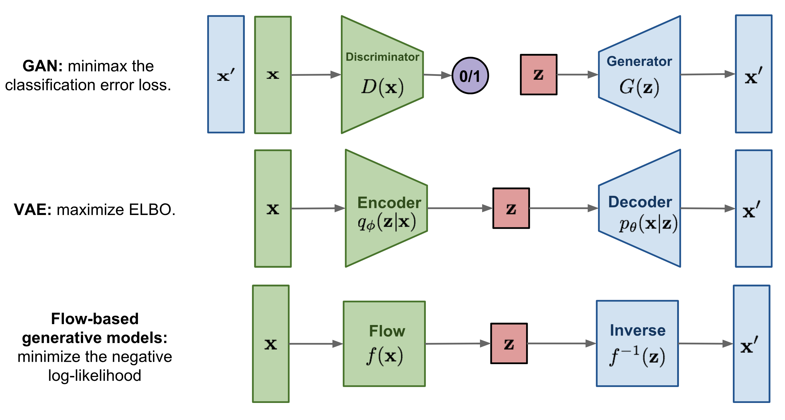 Deep Generative Models from https://lilianweng.github.io/lil-log/2018/10/13/flow-based-deep-generative-models.html
1.2.1. Variational Autoencoder (VAE)
Recall autoencoders (AEs) are deep nerual network models compraised of:
Encoding function:
$$ f_\phi(\mathbf{x}) = \sigma(\mathbf{Wx} + \mathbf{b}) = \mathbf{z}$$
Decoding function:
$$ g_\theta(\mathbf{z}) = \sigma(\mathbf{W'z} + \mathbf{b'}) = \mathbf{x'}$$
Objective/Loss function (reconstruction loss): $$ L(\mathbf{x}, \mathbf{x'}) = ||\mathbf{x} - \mathbf{x'}||^2 $$
VAE (Kingma & Welling, 2014) introduces:
- Probabilistic encoder $q_\phi(\mathbf{z}|\mathbf{x})$ and decoder $p_\theta(\mathbf{x}|\mathbf{z})$
- A prior probability distribution for the latent space: $p_\theta(\mathbf{z})$
- Latent loss defined by Kullback-Leibler divergence: $D_{KL}(q_\phi(\mathbf{z} | \mathbf{x}) \Vert p_\theta(\mathbf{z} | \mathbf{x}))$ to quantify the distance between these two probability distributions
Therefore, the loss function for VAE is composed of the reconstruction loss and the KL-divergence:
$$L_{VAE} = ||\mathbf{x} - \mathbf{x'}||^2 + D_{KL}(q_\phi(\mathbf{z} | \mathbf{x}) \Vert p_\theta(\mathbf{z} | \mathbf{x}))$$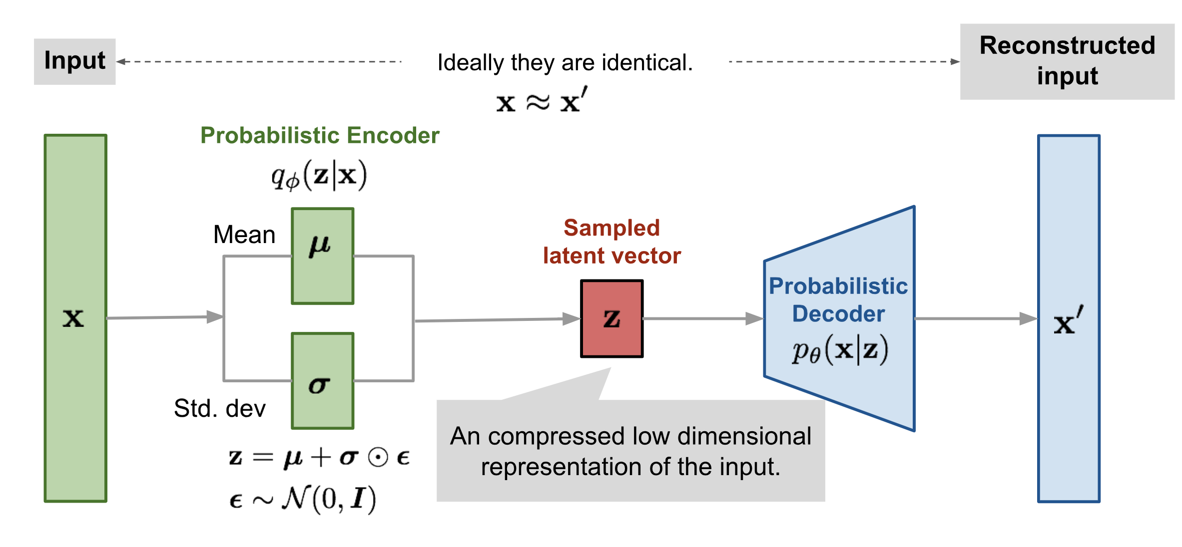 VAE illustration from https://lilianweng.github.io/lil-log/2018/08/12/from-autoencoder-to-beta-vae.html
1.2.2. Generative Adversarial Networks (GANs)
Introduced by Goodfellow et al., in 2014. GAN is composed of a pair of Generative($G$) and Discriminator ($D$) using adversarial training to play a minimax game between G and D.
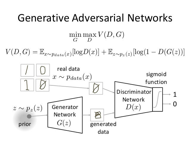 Source: https://www.slideshare.net/ckmarkohchang/generative-adversarial-networks
Many variants of GANs have been developed:
- Bidirectional GAN (BiGAN)
- CycleGAN
- InfoGAN
- Wasserstein GAN
- and many more...
Bidirectional GAN (BiGAN) is particularly attractive in that it explicitly learn a Encoder network to map the input back to the latent space:
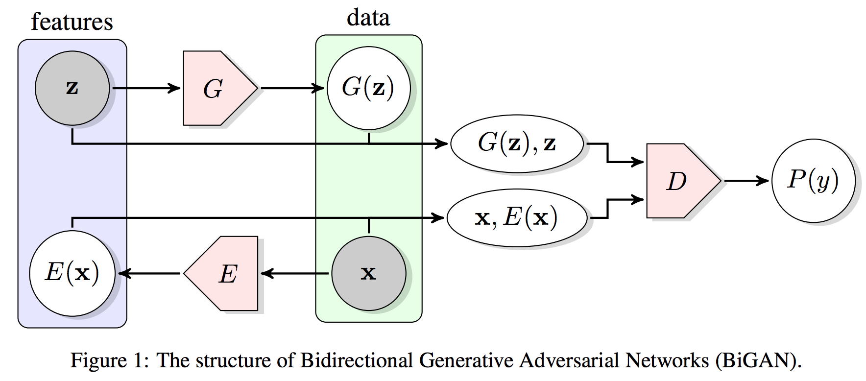 Donahue et al: Adversarial Feature Learning
2. Use of Generative Models
Learns (low dimensional) probability distribution for samples of different classes
- Classification, e.g. predicting cell types based on gene expression vector
- Generates synthetic samples for different classes by sampling the latent space, e.g. generate synthetic gene expression profiles for T-cells
Perform interpolation of samples along different axis
- Find the intermediate states between samples from two classes
- Defines intermediate states along a cell differentiation process
- Estimate psudotime for intermediate cells (from scRNA-seq) along a differentiation axis
- Manipulate a sample along an arbitrary axis
- manipulate faces
- Interesting biological axes:
- Age
- Stemness
- Diseasedness
- Chemical/Genetic perturbations
- Find the intermediate states between samples from two classes
How does the interpolation work?
Centoid of all class $a$ training samples in the latent space: $$ \mathbf{\overline{z}_a} = \frac{1}{m} \sum_{i=0}^m encode(\mathbf{x}_{a,i}) $$
Centoid of all class $b$ training samples in the latent space: $$ \mathbf{\overline{z}_b} = \frac{1}{n} \sum_{i=0}^n encode(\mathbf{x}_{b,i}) $$
The interpolation vector $\mathbf{z_{b \rightarrow a}}$ in the latent space from class $b$ to class $a$: $$ \mathbf{z_{b \rightarrow a}} = \mathbf{\overline{z}_a} - \mathbf{\overline{z}_b} $$
Given any input vector of any class $\mathbf{x_c}$, we can manipulate the input with the interpolation vector by:
$$ \mathbf{z_c} = encode(\mathbf{x_c}) $$$$ \mathbf{x_c'} = decode(\mathbf{z_c} + \alpha \mathbf{z_{b \rightarrow a}})$$3. Experiments of Generative Models with MNIST Data
Steps:
- Fit generative models
- Evaluate learned latent representations of MNIST data
- Dimensionality Reduction
- Generated data from the latent space (z)
- Interpolation in the latent space
- From one class to annother
- Manipulate class c along the a -> b vector
Generative models experimented:
# Load the MNIST data
mnist = input_data.read_data_sets('MNIST_data', one_hot=False)
Extracting MNIST_data/train-images-idx3-ubyte.gz Extracting MNIST_data/train-labels-idx1-ubyte.gz Extracting MNIST_data/t10k-images-idx3-ubyte.gz Extracting MNIST_data/t10k-labels-idx1-ubyte.gz
X_train, X_test = mnist.train.images, mnist.test.images
print (X_train.shape, X_test.shape)
labels_train = mnist.train.labels
n_samples = int(mnist.train.num_examples)
(55000, 784) (10000, 784)
'''Functions to qualitatively and quantitatively evaluate the interpolation effects
'''
def interpolate_from_a_to_b(Z, labels, generator, a, b,
alphas=np.linspace(-3, 3, 10),
figsize=(14,5)
):
'''Interpolation between two classes a and b.
Z: np.array of the latent space with shape: (n_samples, latent_dim)
labels: array of class labels (n_samples, )
'''
# Find the centroids of the classes a, b
z_a_avg = Z[labels == a].mean(axis=0)
z_b_avg = Z[labels == b].mean(axis=0)
# Pick the medoid for class a for interpolation
z_a_med = np.median(Z[labels == a], axis=0)
# The interpolation vector pointing from b -> a
z_b2a = z_a_avg - z_b_avg
x_gens = []
for alpha in alphas:
z_interp = z_a_med + alpha * z_b2a
x_gens.append(generator.generate(z_interp.reshape(1, -1)))
ax = display_mnist_images(x_gens, figsize=figsize)
return ax, x_gens
def interpolate_from_a_to_b_for_c(Z, labels, generator, a, b, c,
alphas=np.linspace(-3, 3, 10),
figsize=(14,5)
):
'''Interpolation between two classes a and b for annother class c.
Z: np.array of the latent space with shape: (n_samples, latent_dim)
labels: array of class labels (n_samples, )
'''
# Find the centroids of the classes a, b
z_a_avg = Z[labels == a].mean(axis=0)
z_b_avg = Z[labels == b].mean(axis=0)
# Find the medoid for class c
z_c_med = np.median(Z[labels == c], axis=0)
# The interpolation vector pointing from b -> a
z_b2a = z_a_avg - z_b_avg
x_gens = []
for alpha in alphas:
z_interp = z_c_med + alpha * z_b2a
x_gens.append(generator.generate(z_interp.reshape(1, -1)))
ax = display_mnist_images(x_gens, figsize=figsize)
return ax, x_gens
def plot_alphas_vs_probas(xs, alphas, discriminator, classes=[]):
'''Plot the predicted probabilities for classes from the discriminator.
xs: 2nd output from `interpolate_from_a_to_b` or `interpolate_from_a_to_b_for_c`
alphas: array of alphas
'''
xs = np.array(xs)[:, 0, :]
xs_pred_probas = discriminator.predict_proba(xs)
fig, ax = plt.subplots()
for c in classes:
ax.plot(alphas, xs_pred_probas[:, c], label=str(c))
ax.legend(loc='best')
ax.set_ylabel('Probability')
ax.set_xlabel('alpha')
return ax
Naive Bayes
gnb = naive_bayes.GaussianNB()
gnb.fit(X_train, labels_train)
GaussianNB(priors=None)
# Learned priors for each class
gnb.class_prior_
array([ 0.09898182, 0.11234545, 0.09945455, 0.10250909, 0.09649091,
0.09067273, 0.09849091, 0.10390909, 0.09798182, 0.09916364])
# Learned mean of each feature per class
gnb.theta_.shape
(10, 784)
# Examine learned average for each digit
for i in range(10):
ax = display_mnist_image(gnb.theta_[i].reshape(1, -1), figsize=(2,2))
ax.set_title('NB learned mean for digit %d' % i)


acc = metrics.accuracy_score(mnist.test.labels, gnb.predict(X_test))
print('Accuracy: %.4f'%acc)
Accuracy: 0.5492
# Compare with a simple Logistic Regression
logit = linear_model.LogisticRegression()
logit.fit(X_train, labels_train)
acc = metrics.accuracy_score(mnist.test.labels, logit.predict(X_test))
print('Accuracy (Logistic Regression): %.4f'%acc)
Accuracy (Logistic Regression): 0.9198
# A hack for Naive Bayes.
# Because the latent space of NB is the identical to original space,
# .generate() method should return identity
gnb.generate = lambda x: x
alphas = np.linspace(-3, 3, 20)
ax, x_gens = interpolate_from_a_to_b(X_test, mnist.test.labels, gnb, 0, 6, alphas=alphas)
ax2 = plot_alphas_vs_probas(x_gens, alphas, logit, classes=[0,6])


ax, x_gens = interpolate_from_a_to_b_for_c(X_test, mnist.test.labels, gnb, 0, 6, 7,
alphas=alphas)
ax2 = plot_alphas_vs_probas(x_gens, alphas, logit, classes=[0,6,7])


VAE
from autoencoder_models.VariationalAutoencoder import VariationalAutoencoder
# Load trained VAE models
vae2d = VariationalAutoencoder.load('trained_models/VAE_2d/')
vae20d = VariationalAutoencoder.load('trained_models/VAE_20d/')
INFO:tensorflow:Restoring parameters from trained_models/VAE_2d/model.ckpt INFO:tensorflow:Restoring parameters from trained_models/VAE_20d/model.ckpt
print(vae2d.n_layers)
print(vae20d.n_layers)
[784, 500, 500, 2] [784, 500, 500, 20]
# Uses trained VAE to transform MNIST into latent spaces
Z_vae2d = vae2d.transform(X_train)
Z_test_vae2d = vae2d.transform(X_test)
print (Z_vae2d.shape, Z_test_vae2d.shape)
Z_vae20d = vae20d.transform(X_train)
Z_test_vae20d = vae20d.transform(X_test)
print (Z_vae20d.shape, Z_test_vae20d.shape)
(55000, 2) (10000, 2) (55000, 20) (10000, 20)
ax = plot_embed(Z_vae2d, labels_train)
ax.set_title('VAE 2d');

ax = plot_embed(decomposition.PCA(n_components=2).fit_transform(Z_vae20d), labels_train)
ax.set_title('VAE 20d -> PCA');

ax = plot_embed(Z_vae20d[:, :2], labels_train)
ax.set_title('VAE 20d -> first 2 dims');

ax = plot_embed(Z_test_vae2d, mnist.test.labels)
ax.set_title('VAE 2d Holdout set');

# Uniformly sample the VAE 2d space
nx = ny = 20
x_values = np.linspace(-3, 3, nx)
y_values = np.linspace(-3, 3, ny)
z_uniform = np.empty((nx, ny, 2))
canvas = np.empty((28*ny, 28*nx))
for i, yi in enumerate(x_values):
for j, xi in enumerate(y_values):
z_mu = np.array([[xi, yi]])
x_mean = vae2d.generate(z_mu)
canvas[(nx-i-1)*28:(nx-i)*28, j*28:(j+1)*28] = x_mean[0].reshape(28, 28)
fig, ax = plt.subplots(figsize=(10,10))
ax.imshow(canvas, origin="upper", cmap="gray")
ax.set_axis_off()

# Random normal sampling of the VAE 20d space
canvas = sample_latent_space(vae20d, 20, sample_type='normal')
print(canvas.shape)
fig, ax = plt.subplots(figsize=(10,10))
ax.imshow(canvas, origin="upper", cmap="gray")
ax.set_axis_off()
(560, 560)

# Generate averages (centroid) of the digits in latent space (VAE 2d)
for i in range(10):
z_i_avg = Z_vae2d[labels_train == i].mean(axis=0).reshape(1, -1)
ax = display_mnist_image(vae2d.generate(z_i_avg), figsize=(2,2))
ax.set_title('Centoid %d' % i)


# Generate averages (centroid) of the digits in latent space (VAE 20d)
for i in range(10):
z_i_avg = Z_vae20d[labels_train == i].mean(axis=0).reshape(1, -1)
ax = display_mnist_image(vae20d.generate(z_i_avg), figsize=(2,2))
ax.set_title('Centoid %d' % i)


alphas = np.linspace(-3, 3, 20)
ax, x_gens = interpolate_from_a_to_b(Z_test_vae2d, mnist.test.labels, vae2d,
0, 6,
alphas=alphas)
ax.set_title('VAE 2d')
ax2 = plot_alphas_vs_probas(x_gens, alphas, logit, classes=[0,6])
ax2.set_title('VAE 2d')
Text(0.5,1,'VAE 2d')


alphas = np.linspace(-5, 5, 20)
ax, x_gens = interpolate_from_a_to_b_for_c(Z_test_vae2d, mnist.test.labels, vae2d,
0, 6, 7,
alphas=alphas)
ax.set_title('VAE 2d')
ax2 = plot_alphas_vs_probas(x_gens, alphas, logit, classes=[0,6,7])
ax2.set_title('VAE 2d')
Text(0.5,1,'VAE 2d')


alphas = np.linspace(-3, 3, 20)
ax, x_gens = interpolate_from_a_to_b(Z_test_vae20d, mnist.test.labels, vae20d,
0, 6,
alphas=alphas)
ax.set_title('VAE 20d')
ax2 = plot_alphas_vs_probas(x_gens, alphas, logit, classes=[0,6])
ax2.set_title('VAE 20d')
Text(0.5,1,'VAE 20d')


alphas = np.linspace(-5, 5, 20)
ax, x_gens = interpolate_from_a_to_b_for_c(Z_test_vae20d, mnist.test.labels, vae20d,
0, 6, 7,
alphas=alphas)
ax.set_title('VAE 20d')
ax2 = plot_alphas_vs_probas(x_gens, alphas, logit, classes=[0,6,7])
ax2.set_title('VAE 20d')
Text(0.5,1,'VAE 20d')


Use VAE to perform interpolation between all (45) pairs of digits
alphas = np.linspace(-1, 0, 30)
n = 45
canvas = np.empty((28*n, 28*len(alphas))) # To collect all the generated images
i = 0
for digit_i, digit_j in combinations(range(10), 2):
ax, x_gens = interpolate_from_a_to_b(Z_test_vae20d, mnist.test.labels, vae20d,
digit_i, digit_j,
alphas=alphas)
ax.set_title('%d -> %d' % (digit_j, digit_i) )
for j in range(len(alphas)):
x = x_gens[j]
x = preprocessing.minmax_scale(x.T).T
canvas[(i)*28:(i+1)*28, j*28:(j+1)*28] = x.reshape(28, 28)
i += 1


fig, ax = plt.subplots(figsize=(12,16))
ax.imshow(canvas, cmap="gray")
ax.set_axis_off()
ax.set_title('Interpolations in the latent space of VAE');

BiGAN
from keras_gan.bigan import BiGAN
Using TensorFlow backend.
bigan = BiGAN.load('trained_models/bigan_20/')
bigan.params
{'g_n_layers': [784, 500, 500, 20],
'd_n_layers': [1000, 1000, 1000],
'learning_rate': 0.0002}
canvas = sample_latent_space(bigan, 20, sample_type='normal')
print(canvas.shape)
fig, ax = plt.subplots(figsize=(10,10))
ax.imshow(canvas, origin="upper", cmap="gray")
ax.set_axis_off()
(560, 560)

Z_gan20d = bigan.transform(X_train)
Z_test_gan20d = bigan.transform(X_test)
print (Z_gan20d.shape, Z_test_gan20d.shape)
(55000, 20) (10000, 20)
ax = plot_embed(decomposition.PCA(n_components=2).fit_transform(Z_gan20d), labels_train)
ax.set_title('BiGAN 20d -> PCA');

# Generate averages (centroid) of the digits in latent space (BiGAN 20d)
for i in range(10):
z_i_avg = Z_gan20d[labels_train == i].mean(axis=0).reshape(1, -1)
ax = display_mnist_image(bigan.generate(z_i_avg), figsize=(2,2))
ax.set_title('Centoid %d' % i)


alphas = np.linspace(-3, 3, 20)
ax, x_gens = interpolate_from_a_to_b(Z_test_gan20d, mnist.test.labels, bigan,
0, 6,
alphas=alphas)
ax.set_title('BiGAN 20d')
ax2 = plot_alphas_vs_probas(x_gens, alphas, logit, classes=[0,6])
ax2.set_title('BiGAN 20d')
Text(0.5,1,'BiGAN 20d')


alphas = np.linspace(-5, 5, 20)
ax, x_gens = interpolate_from_a_to_b_for_c(Z_test_gan20d, mnist.test.labels, bigan,
0, 6, 7,
alphas=alphas)
ax.set_title('BiGAN 20d')
ax2 = plot_alphas_vs_probas(x_gens, alphas, logit, classes=[0,6,7])
ax2.set_title('BiGAN 20d')
Text(0.5,1,'BiGAN 20d')


References:
- Ng AY & Jordan MI: On Discriminative vs. Generative classifiers
- Kingma & Welling: Auto-Encoding Variational Bayes
- Goodfellow IJ et al: Generative Adversarial Networks
- Donahue et al: Adversarial Feature Learning
- [Flow-based Deep Generative Models
](https://lilianweng.github.io/lil-log/2018/10/13/flow-based-deep-generative-models.html)