 CS 236756 - Technion - Intro to Machine Learning
 Agenda
In [1]:
# imports for the tutorial
import numpy as np
import pandas as pd
import matplotlib.pyplot as plt
from mpl_toolkits.mplot3d import Axes3D
%matplotlib notebook
 Optimization Problems
 Definitions
- Objective Function - mathematical function which is optimized by changing the values of the design variables.
- Design Variables - variables that we, as designers, can change.
- Constraints - functions of the design variables which establish limits in individual variables or combinations of design.
- For example - "Find $\theta$ that minimizes $f_{\theta}(x)$ s.t. (subject to) $\theta \leq 1$"
The main problem in optimization is how to search for the values of decision variables that minimize the cost/objective function.
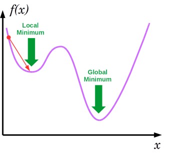
Types of Objective Functions
- Unimodal - only one optimum, that is, the local optimum is also global.

- Multimodal - more than one optimum
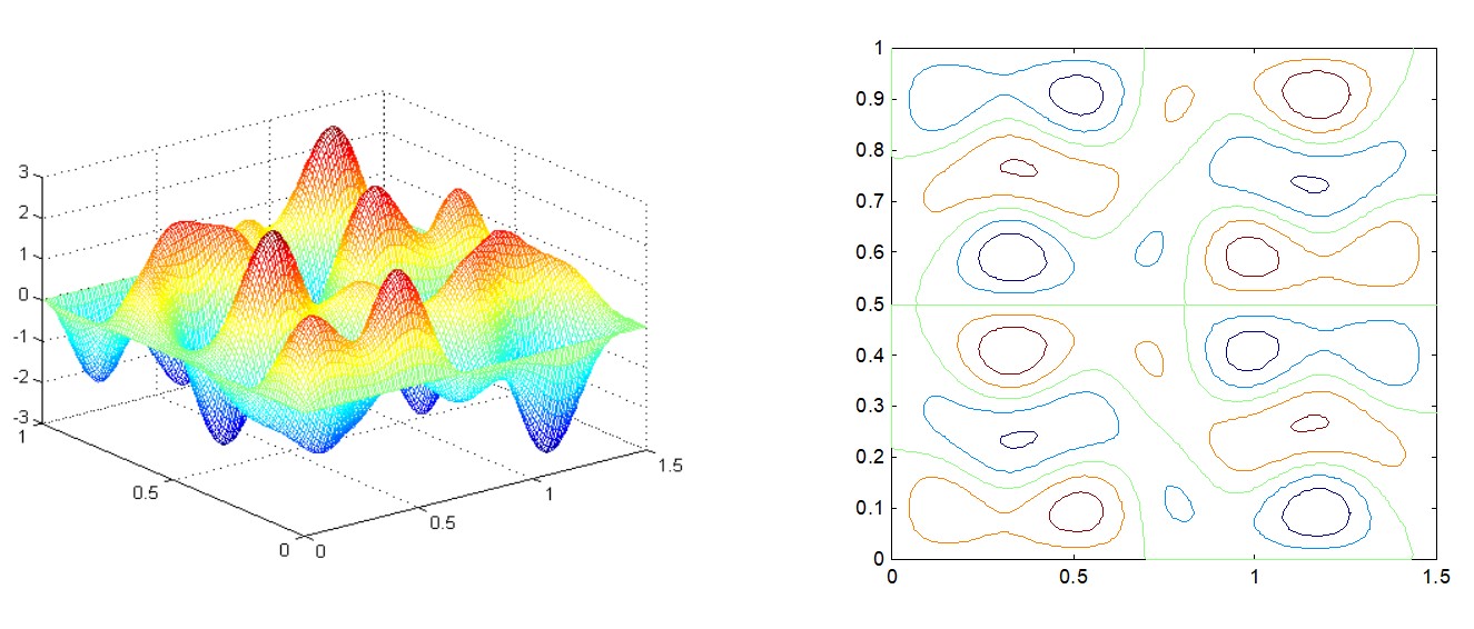
Most search schemes are based on the assumption of unimodal surface. The optimum determined in such cases is called local optimum design.
The global optimum is the best of all local optimum designs.
 Convexity
- Definition: $$\forall x_1, x_2 \in X, \forall t \in [0,1]: $$ $$ f(tx_1 + (1-t)x_2) \leq tf(x_1) + (1-t)f(x_2) $$
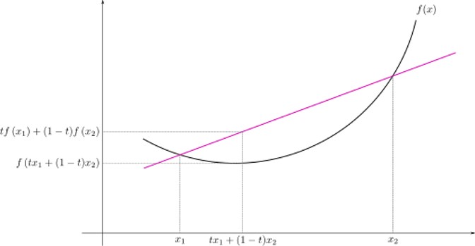
- Convex functions are unimodal
 Continuous Optimization
- Derivative based optimization - the search directions are determined based on deivative information
- Methods include:
- Gradient Descent
- Newton method
- Conjugate gradient
- We will focus on Gradient Descent
 1-D Optimization
 (Batch) Gradient Descent
- Generic optimization algorithm capable of finding optimal solutions to a wide range of problems.
- The general idea is to tweak parameters iteratively to minimize a cost function.
- It measures the local gradient of the error function with regards to the parameter vector ($\theta$ or $w$), and it goes down in the direction of the descending gradient. Once the gradient is zero - the minimum is reached (=convergence).
- Learning Rate hyperparameter - it is the size of step to be taken in each iteration.
- Too small $\rightarrow$ the algorithm will have to go through many iterations to converge, which will take a long time
- Too high $\rightarrow$ might make the algorithm diverge as it may miss the minimum
 Image Source
- Pseudocode:
- Require: Learning rate $\alpha_k$
- Require: Initial parameter $w$
- While stopping criterion not met do
- Compute gradient: $g \leftarrow f'(x,w)$ (more specifically, for $M$ samples: $g \leftarrow \frac{1}{M}\sum_{i=1}^M f'(x_i,w)$, where $f'$ is w.r.t $\theta$ or $w$)
- Apply update: $w \leftarrow w - \alpha_k g$
- $k \leftarrow k + 1$
- end while
- Visualization:
- Convergene: When the cost function is convex and its slope does not change abruptly, (Batch) GD with a fixed learning rate will eventually converge to the optimal solution (but the time is depndent on the rate).
 Example - Linear Least Squares
- Problem Formulation
- $y \in \mathbb{R}^N$ - vector of values
- $X \in \mathbb{R}^N$ - data matrix with one feature (= data vector)
- $w \in \mathbb{R}$ - the parameter to be learnt
- Goal: find $w$ that best fits the measurement y
- Mathematically:
- In vector form:
 LLS - Analytical Solution
- Mathematically:
- The derivative:
- The second derivative, to ensure minimum:
In [2]:
# generate some random data
N = 20
x = np.linspace(1, 20, N)
y = 5 * x + np.random.randn(N)
In [3]:
# lls - analytical solution
# we want to find w that minimizes (wx-y)^2
# by the above derivation
w = np.sum(y * x) / np.sum(np.square(x))
print("best w:", w)
best w: 4.973943975346493
In [4]:
def plot_lls_sol(x, y, w, title=""):
    fig = plt.figure(figsize=(8,5))
    ax = fig.add_subplot(1,1,1)
    ax.scatter(x, y, label="y")
    ax.plot(x, w * x, label="wx", color='r')
    ax.legend()
    ax.grid()
    ax.set_xlabel("x")
    ax.set_title(title)
In [5]:
# let's plot
plot_lls_sol(x, y, w, "Analytical Solution for min(wx-y)^2")

LLS - Gradient Descent Solution
- Pseudocode:
- Require: Learning rate $\alpha_k$
- Require: Initial parameter $w$
- While stopping criterion not met do
- Compute gradient: $g \leftarrow \frac{1}{N}\sum_{i=1}^N 2wx_i^2 -2x_iy_i$
- Apply update: $w \leftarrow w - \alpha_k g$
- $k \leftarrow k + 1$
- end while
In [6]:
# lls - gradient descent solution
N = 20 # num samples
num_iterations = 20
alpha_k = 0.005
# we want to find w that minimizes (wx-y)^2
# initialize w
w = 0
for i in range(num_iterations):
    print("iter:", i, " w = ", w)
    gradient = np.sum(2 * w * np.square(x) - 2 * x * y) / N
    w = w - alpha_k * gradient
print("best w:", w)
iter: 0  w =  0
iter: 1  w =  7.1376096046222175
iter: 2  w =  4.032749426611554
iter: 3  w =  5.383363604046192
iter: 4  w =  4.795846436862124
iter: 5  w =  5.051416404587194
iter: 6  w =  4.940243468626789
iter: 7  w =  4.988603695769565
iter: 8  w =  4.967566996962457
iter: 9  w =  4.9767179609435495
iter: 10  w =  4.972737291611774
iter: 11  w =  4.974468882771096
iter: 12  w =  4.973715640616791
iter: 13  w =  4.974043300953914
iter: 14  w =  4.973900768707265
iter: 15  w =  4.973962770234557
iter: 16  w =  4.973935799570186
iter: 17  w =  4.973947531809187
iter: 18  w =  4.973942428285222
iter: 19  w =  4.973944648318146
best w: 4.973943682603824
In [7]:
plot_lls_sol(x, y, w, "Gradient Descent Solution for min(wx-y)^2")

- Least Squares Visualization:
 Stochastic Gradient Descent (Mini-Batch Gradient Descent)
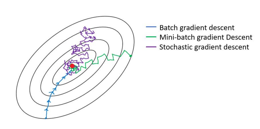
- The main problem with (Batch) GD is that it uses the whole training set to compute the gradients. But what if that training set is huge? Computing the gradient can take a very long time.
- Stochastic Gradient Descent on the other hand, samples just one instance randomly at every step and computes the gradients based on that single instance. This makes the algorithm much faster but due to its randomness, it is much less stable. Instead of steady decreasing untill reaching the minimum, the cost function will bounce up and down, decreasing only on average. With time, it will get very close to the minimum, but once it is there it will continue to bounce around!
- The final parameters are good but not optimal.
- When the cost function is very irregular, this bouncing can actually help the algorithm escape local minima, so SGD has better chance to find the global minimum.
- How to find optimal parameters using SGD?
- Reduce the learning rate gradually: this is called learning schedule
- But don't reduce too quickly or you will get stuck at a local minimum or even frozen!
- Reduce the learning rate gradually: this is called learning schedule
- Mini-Batch Gradient Descent - same idea as SGD, but instead of one instance each step, $m$ samples.
- Get a little bit closer to the minimum than SGD but a little harder to escape local minima.
- Pseudocode:
- Require: Learning rate $\alpha_k$
- Require: Initial parameter $w$
- While stopping criterion not met do
- Sample a minibatch of $m$ examples from the training set ($m=1$ for SGD)
- Set $\{x_1,...,x_m,\}$ with corresponding targets $\{y_1,...,y_m\}$
- Compute gradient: $g \leftarrow \frac{1}{m} \sum_{i=1}^m f'(x_i,w)$
- Apply update: $w \leftarrow w - \alpha_k g$
- $k \leftarrow k + 1$
- end while
In [8]:
def batch_generator(x, y, batch_size, shuffle=True):
    """
    This function generates batches for a given dataset x.
    """
    N = len(x)
    num_batches = N // batch_size
    batch_x = []
    batch_y = []
    if shuffle:
        # shuffle
        rand_gen = np.random.RandomState(0)
        shuffled_indices = rand_gen.permutation(np.arange(len(x)))
        x = x[shuffled_indices]
        y = y[shuffled_indices]
    for i in range(N):
        batch_x.append(x[i])
        batch_y.append(y[i])
        if len(batch_x) == batch_size:
            yield np.array(batch_x), np.array(batch_y)
            batch_x = []
            batch_y = []
    if batch_x:
        yield np.array(batch_x), np.array(batch_y)
In [9]:
# mini-batch gradient descent
batch_size = 5
num_batches = N // batch_size
print("total batches:", num_batches)
num_iterations = 20
alpha_k = 0.001
batch_gen = batch_generator(x, y, batch_size, shuffle=True)
# we want to find w that minimizes (wx-y)^2
# initialize w
w = 0
for i in range(num_iterations):
    for batch_i, batch in enumerate(batch_gen):
        batch_x, batch_y = batch
        if batch_i % 5 == 0:
            print("iter:", i, "batch:", batch_i, " w = ", w)
        gradient = np.sum(2 * w * np.square(batch_x) - 2 * batch_x * batch_y) / len(batch_x)
        w = w - alpha_k * gradient
    batch_gen = batch_generator(x, y, batch_size, shuffle=True)
print("best w:", w)
total batches: 4
iter: 0 batch: 0  w =  0
iter: 1 batch: 0  w =  3.714921791540526
iter: 2 batch: 0  w =  4.660336847464463
iter: 3 batch: 0  w =  4.900936698046245
iter: 4 batch: 0  w =  4.962167252538953
iter: 5 batch: 0  w =  4.9777498923220564
iter: 6 batch: 0  w =  4.981715537654223
iter: 7 batch: 0  w =  4.982724759655079
iter: 8 batch: 0  w =  4.982981597814244
iter: 9 batch: 0  w =  4.983046960876035
iter: 10 batch: 0  w =  4.983063595202728
iter: 11 batch: 0  w =  4.983067828493167
iter: 12 batch: 0  w =  4.983068905828502
iter: 13 batch: 0  w =  4.983069180000908
iter: 14 batch: 0  w =  4.983069249775384
iter: 15 batch: 0  w =  4.983069267532377
iter: 16 batch: 0  w =  4.9830692720513765
iter: 17 batch: 0  w =  4.983069273201423
iter: 18 batch: 0  w =  4.983069273494099
iter: 19 batch: 0  w =  4.983069273568582
best w: 4.983069273587538
In [10]:
# let's plot
plot_lls_sol(x, y, w, "Mini-Batch Gradient Descent Solution for min(wx-y)^2")

GD Comparison Summary
| Method | Accuracy | Update Speed | Memory Usage | Online Learning |
|---|---|---|---|---|
| Batch Gradient Descent | Good | Slow | High | No |
| Stochastic Gradient Descent | Good (with softening) | Fast | Low | Yes |
| Mini-Batch Gradient Descent | Good | Medium | Medium | Yes (depends on the MB size) |
- "Online" - samples arrive while the algorithm runs (that is, when the algorithm starts running, not all samples exist)
- Note: All of the Gradient Descent algorithms require scaling if the feaures are not within the same range!
Challenges
- Choosing a learning rate
- Defining learning schedule
- Working with features of different scales (e.g. heights (cm), weights (kg) and age (scalar))
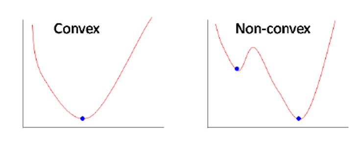
- Avoiding local minima (or suboptimal minima)
 Mathematical Background
 Multivariate Calculus
- The Derivative - the derivative of $f: \mathbb{R} \rightarrow \mathbb{R}$ is a function $f': \mathbb{R} \rightarrow \mathbb{R}$ given by:
* Illustration: <img src="./assets/tut_06_deriv.jpg" style="height:200px">
- Rewrite the above: $$ \lim_{h \to 0} \frac{f(x+h) - f(x) -f'(x) \cdot h}{h}=0$$

- The Gradient - the gradient of $f: \mathbb{R}^N \rightarrow \mathbb{R}$ is a function $\nabla f: \mathbb{R}^N \rightarrow \mathbb{R}^N$ given by: $$ \lim_{h \to 0} \frac{||f(\overline{x}+\overline{h}) - f(\overline{x}) -\nabla f(\overline{x}) \cdot \overline{h}||}{||\overline{h}||} = 0$$

- The gradient can be expressed in terms of the function's partial derivatives: $$\nabla f(x) = \begin{bmatrix} \frac{\partial f}{\partial x_1} \\ \frac{\partial f}{\partial x_2} \\ \vdots \\ \frac{\partial f}{\partial x_n} \end{bmatrix} $$
- Illustration:

- Illustration:
- The Hessian Matrix
- Definition: $H(f)(x)_{i,j} = \frac{\partial^2}{\partial x_i \partial x_j} f(x)$
- $$ \begin{bmatrix} \frac{\partial^2 f}{\partial x_1^2} & \frac{\partial^2 f}{\partial x_1 \partial x_2} & \cdots & \frac{\partial^2 f}{\partial x_1 \partial x_n} \\ \frac{\partial^2 f}{\partial x_2 x_1} & \frac{\partial^2 f}{\partial x_2^2} & \cdots & \frac{\partial^2 f}{\partial x_2 \partial x_n} \\ \vdots & \vdots & \ddots & \vdots \\ \frac{\partial^2 f}{\partial x_n x_1} & \frac{\partial^2 f}{\partial x_n \partial x_2} & \cdots & \frac{\partial^2 f}{\partial x_n^2} \end{bmatrix} $$
 Matrix Calculus - Vector & Matrix Derivatives
- We will use most of the derivations "as is" without derivation.
- A good reference: The Matrix Cookbook
 REMEMBER - ALWAYS write the dimensions of each component and identify whether the expression is a matrix, vector or scalar!
 Derivative of Vector Multiplication
- Let $x, a \in \mathbb{R}^N \rightarrow x, a$ are vectors
- $\frac{\partial x^Ta}{\partial x} = \frac{\partial a^Tx}{\partial x} = a$
- $x^Ta = a^Tx$ are scalars
- $a$ is a vector
- Derivation: $$ f = x^Ta = [x_1, x_2, ..., x_n] \begin{bmatrix} a_{1} \\a_{2} \\ \vdots \\a_{n}\end{bmatrix} = a_1 x_1 + a_2 x_2 + ... + a_n x_n = \sum_{i=1}^n a_i x_i$$ $$\frac{\partial x^Ta}{\partial x} = \begin{bmatrix}\frac{\partial f}{\partial x_1} \\ \frac{\partial f}{\partial x_2} \\ \vdots \\ \frac{\partial f}{\partial x_n} \end{bmatrix} = \begin{bmatrix} a_{1} \\ a_{2} \\ \vdots \\ a_{n} \end{bmatrix} = a $$
 Common Derivations
- $\nabla_x Ax = A^{T}$
- $\nabla_x x^{T} A x = (A + A^{T}) x$
- If $W$ is symetric:
- $\frac{\partial}{\partial s} (x-As)^T W (x-As) = -2A^TW(x-As)$
- $\frac{\partial}{\partial x} (x-As)^T W (x-As) = 2W(x-As)$
- If $W$ is symetric:
- $\frac{\partial}{\partial A} \ln |A| = A^{-T}$
- $\frac{\partial}{\partial A} Tr[AB] = B^{T}$
 The Chain Rule
- Let $$ f(x) = h(g(x))$$ $$x \in \mathbb{R}^n $$ $$ f, g : \mathbb{R}^n \rightarrow \mathbb{R}$$ $$ h: \mathbb{R} \rightarrow \mathbb{R}$$
- $ \nabla f = h' \cdot \nabla g$
 Exercise 1 - The Chain Rule
Find the gradient of $f(x) = \sqrt{x^TQx}$ ($Q$ is positive definite)
Solution 1
- $g(x) = x^TQx \rightarrow \nabla g = (Q + Q^T) x = 2Qx$
- $h(z) = \sqrt{z} \rightarrow h'(z) = \frac{1}{2\sqrt{z}}$
- $\nabla f =\frac{1}{2\sqrt{x^TQx}}2Qx = \frac{Qx}{\sqrt{x^TQx}} $
 Multi-Dimensional Optimization
 Optimality Conditions
- If $f$ has local optimum at $x_0$ then $\nabla f(x_0) = 0$
- If the Hessian is:
- Positive Definite (all eigenvalues positive) at $x_0 \rightarrow$ local minimum
- Negative Definite (all eigenvalues negative) at $x_0 \rightarrow$ local maximum
- Both positive and negative eigenvalues at $x_0 \rightarrow$ saddle point

Example - (Multivariate) Linear Least Squares
- Problem Formulation
- $y \in \mathbb{R}^N$ - vector of values
- $X \in \mathbb{R}^{N \times L}$ - data matrix with $N$ examples and $L$ features
- $w \in \mathbb{R}^L$ - the parameters to be learnt, a weight for each feature
- Goal: find $w$ that best fits the measurement y, that is, find a weighted linear combination of the feature vector to best fit the measurment $y$
- Mathematiacally, the problem is:
- In vector form:
(Multivariate) LLS - Analytical Solution
- Mathematically:
- The derivative:
$$X^TX \in \mathbb{R}^{L \times L} $$
In [11]:
# let's load the cancer dataset
dataset = pd.read_csv('./datasets/cancer_dataset.csv')
# print the number of rows in the data set
number_of_rows = len(dataset)
# reminder, the data looks like this
dataset.sample(10)
Out[11]:
| id | diagnosis | radius_mean | texture_mean | perimeter_mean | area_mean | smoothness_mean | compactness_mean | concavity_mean | concave points_mean | ... | texture_worst | perimeter_worst | area_worst | smoothness_worst | compactness_worst | concavity_worst | concave points_worst | symmetry_worst | fractal_dimension_worst | Unnamed: 32 | |
|---|---|---|---|---|---|---|---|---|---|---|---|---|---|---|---|---|---|---|---|---|---|
| 187 | 874373 | B | 11.71 | 17.19 | 74.68 | 420.3 | 0.09774 | 0.06141 | 0.03809 | 0.03239 | ... | 21.39 | 84.42 | 521.5 | 0.1323 | 0.1040 | 0.1521 | 0.10990 | 0.2572 | 0.07097 | NaN |
| 323 | 895100 | M | 20.34 | 21.51 | 135.90 | 1264.0 | 0.11700 | 0.18750 | 0.25650 | 0.15040 | ... | 31.86 | 171.10 | 1938.0 | 0.1592 | 0.4492 | 0.5344 | 0.26850 | 0.5558 | 0.10240 | NaN |
| 355 | 9010258 | B | 12.56 | 19.07 | 81.92 | 485.8 | 0.08760 | 0.10380 | 0.10300 | 0.04391 | ... | 22.43 | 89.02 | 547.4 | 0.1096 | 0.2002 | 0.2388 | 0.09265 | 0.2121 | 0.07188 | NaN |
| 82 | 8611555 | M | 25.22 | 24.91 | 171.50 | 1878.0 | 0.10630 | 0.26650 | 0.33390 | 0.18450 | ... | 33.62 | 211.70 | 2562.0 | 0.1573 | 0.6076 | 0.6476 | 0.28670 | 0.2355 | 0.10510 | NaN |
| 329 | 895633 | M | 16.26 | 21.88 | 107.50 | 826.8 | 0.11650 | 0.12830 | 0.17990 | 0.07981 | ... | 25.21 | 113.70 | 975.2 | 0.1426 | 0.2116 | 0.3344 | 0.10470 | 0.2736 | 0.07953 | NaN |
| 80 | 861103 | B | 11.45 | 20.97 | 73.81 | 401.5 | 0.11020 | 0.09362 | 0.04591 | 0.02233 | ... | 32.16 | 84.53 | 525.1 | 0.1557 | 0.1676 | 0.1755 | 0.06127 | 0.2762 | 0.08851 | NaN |
| 530 | 91858 | B | 11.75 | 17.56 | 75.89 | 422.9 | 0.10730 | 0.09713 | 0.05282 | 0.04440 | ... | 27.98 | 88.52 | 552.3 | 0.1349 | 0.1854 | 0.1366 | 0.10100 | 0.2478 | 0.07757 | NaN |
| 486 | 913102 | B | 14.64 | 16.85 | 94.21 | 666.0 | 0.08641 | 0.06698 | 0.05192 | 0.02791 | ... | 25.44 | 106.00 | 831.0 | 0.1142 | 0.2070 | 0.2437 | 0.07828 | 0.2455 | 0.06596 | NaN |
| 9 | 84501001 | M | 12.46 | 24.04 | 83.97 | 475.9 | 0.11860 | 0.23960 | 0.22730 | 0.08543 | ... | 40.68 | 97.65 | 711.4 | 0.1853 | 1.0580 | 1.1050 | 0.22100 | 0.4366 | 0.20750 | NaN |
| 48 | 857155 | B | 12.05 | 14.63 | 78.04 | 449.3 | 0.10310 | 0.09092 | 0.06592 | 0.02749 | ... | 20.70 | 89.88 | 582.6 | 0.1494 | 0.2156 | 0.3050 | 0.06548 | 0.2747 | 0.08301 | NaN |
10 rows × 33 columns
In [32]:
def plot_3d(x, y, z):
    %matplotlib notebook
    fig = plt.figure(figsize=(5, 5))
    ax = fig.add_subplot(111, projection='3d')
    ax.scatter(x, y, z)
    ax.set_xlabel('Radius Mean')
    ax.set_ylabel('Area Mean')
    ax.set_zlabel('Perimeter Mean')
    ax.set_title("Breast Cancer - Radius Mean vs. Area Mean vs. Perimeter Mean")
In [33]:
# let's plot X = [radius, area], y = perimeter
xs = dataset[['radius_mean']].values
ys = dataset[['area_mean']].values
zs = dataset[['perimeter_mean']].values
plot_3d(xs, ys, zs)

In [34]:
def plot_3d_lls(x, y, z, lls_sol, title=""):
    # plot
    %matplotlib notebook
    fig = plt.figure(figsize=(5, 5))
    ax = fig.add_subplot(111, projection='3d')
    ax.scatter(x, y, z, label='Y')
    ax.scatter(x, y, lls_sol, label='Xw')
    ax.legend()
    ax.set_xlabel('Radius Mean')
    ax.set_ylabel('Area Mean')
    ax.set_zlabel('Perimeter Mean')
    ax.set_title(title)
In [35]:
# multivariate lls - analytical solution
X = dataset[['radius_mean', 'area_mean']].values
Y = dataset[['perimeter_mean']].values
xs = dataset[['radius_mean']].values
ys = dataset[['area_mean']].values
zs = dataset[['perimeter_mean']].values
w = np.linalg.inv(X.T @ X) @ X.T @ Y
lls_sol = X @ w
print("w:")
print(w)
w:
[[6.19721311]
 [0.00676913]]
In [36]:
# plot
plot_3d_lls(xs, ys, zs, lls_sol, "Breast Cancer - Radius Mean vs. Area Mean vs. Perimeter Mean - LLS Analyitical")

What If L is Very Large???
If $L = 1000$, we would need to invert a $1000 \times 1000$ matrix, which would take about $10^9$ operations!
(Batch) Gradient Descent
- Pseudocode:
- Require: Learning rate $\alpha_k$
- Require: Initial parameter vector $w$
- While stopping criterion not met do
- Compute gradient: $g \leftarrow \nabla f(x,w)$
- Apply update: $w \leftarrow w - \alpha_k g$
- $k \leftarrow k + 1$
- end while
- For Linear Least Squares:
- Require: Learning rate $\alpha_k$
- Require: Initial parameter vector $w$
- While stopping criterion not met do
- Compute gradient: $g \leftarrow 2X^TXw - 2X^Ty$
- Apply update: $w \leftarrow w - \alpha_k g$
- $k \leftarrow k + 1$
- end while
In [ ]:
# multivariate lls - gradient descent solution
X = dataset[['radius_mean', 'area_mean']].values
Y = dataset[['perimeter_mean']].values
# Scaling
X = (X - X.mean(axis=0, keepdims=True)) / X.std(axis=0, keepdims=True)
Y = (Y - Y.mean(axis=0, keepdims=True)) / Y.std(axis=0, keepdims=True)
num_iterations = 20
alpha_k = 0.0001
L = X.shape[1]
# initialize w
w = np.zeros((L, 1))
for i in range(num_iterations):
    print("iter:", i, " w = ")
    print(w)
    gradient = 2 * X.T @ X @ w - 2 * X.T @ Y
    w = w - alpha_k * gradient
lls_sol = X @ w
print("w:")
print(w)
In [38]:
# plot
plot_3d_lls(X[:,0], X[:, 1], Y, lls_sol, "Breast Cancer - Radius Mean vs. Area Mean vs. Perimeter Mean - LLS GD")

Stochastic Gradient Descent (Mini-Batch Gradient Descent)
- Pseudocode:
- Require: Learning rate $\alpha_k$
- Require: Initial parameter $w$
- While stopping criterion not met do
- Sample a minibatch of $m$ examples from the training set ($m=1$ for SGD)
- Set $\tilde{X} = [x_1,...,x_m] $ with corresponding targets $\tilde{Y} = [y_1,...,y_m]$
- Compute gradient: $g \leftarrow 2\tilde{X}^T\tilde{X} - 2\tilde{X}^T \tilde{Y}$
- Apply update: $w \leftarrow w - \alpha_k g$
- $k \leftarrow k + 1$
- end while
In [19]:
def batch_generator(x, y, batch_size, shuffle=True):
    """
    This function generates batches for a given dataset x.
    """
    N, L = x.shape
    num_batches = N // batch_size
    batch_x = []
    batch_y = []
    if shuffle:
        # shuffle
        rand_gen = np.random.RandomState(0)
        shuffled_indices = rand_gen.permutation(np.arange(N))
        x = x[shuffled_indices, :]
        y = y[shuffled_indices, :]
    for i in range(N):
        batch_x.append(x[i, :])
        batch_y.append(y[i, :])
        if len(batch_x) == batch_size:
            yield np.array(batch_x).reshape(batch_size, L), np.array(batch_y).reshape(batch_size, 1)
            batch_x = []
            batch_y = []
    if batch_x:
        yield np.array(batch_x).reshape(-1, L), np.array(batch_y).reshape(-1, 1)
In [29]:
# multivaraite mini-batch gradient descent
X = dataset[['radius_mean', 'area_mean']].values
Y = dataset[['perimeter_mean']].values
# Scaling
X = (X - X.mean(axis=0, keepdims=True)) / X.std(axis=0, keepdims=True)
Y = (Y - Y.mean(axis=0, keepdims=True)) / Y.std(axis=0, keepdims=True)
N = X.shape[0]
batch_size = 10
num_batches = N // batch_size
print("total batches:", num_batches)
total batches: 56
In [ ]:
num_iterations = 10
alpha_k = 0.001
batch_gen = batch_generator(X, Y, batch_size, shuffle=True)
# initialize w
w = np.zeros((L, 1))
for i in range(num_iterations):
    for batch_i, batch in enumerate(batch_gen):
        batch_x, batch_y = batch
        if batch_i % 50 == 0:
            print("iter:", i, "batch:", batch_i, " w = ")
            print(w)
        gradient = 2 * batch_x.T @ batch_x @ w - 2 * batch_x.T @ batch_y
        w = w - alpha_k * gradient
    batch_gen = batch_generator(X, Y, batch_size, shuffle=True)

lls_sol = X @ w
In [31]:
# plot
plot_3d_lls(X[:,0], X[:, 1], Y, lls_sol, "Breast Cancer - Radius Mean vs. Area Mean vs. Perimeter Mean - LLS Mini-Batch GD")
print("w:")
print(w)

w:
[[0.55894282]
 [0.42792729]]
 Constrained Optimization
 Largrange Multipliers
- A method for optimization with equality constraints
- The general case: $$ \min f(x,y) $$ $$ \textit{s.t. (subject to)}: g(x,y)=0 $$
- The Lagrange function (Lagrangian) is defined by: $$ \mathcal{L}(x,y,\lambda) = f(x,y) -\lambda \cdot g(x,y) $$
- Geometric Intuition: let's look at the following figure where we wish to maximize $f(x,y)$ s.t $g(x,y)=0$ -

- To maximize $f(x,y)$ subject to $g(x,y)=0$ is to find the largest value $c \in \{7,8,9,10,11\}$ such that the level curve (contour) $f(x,y) = c$ intersects with $g(x,y)=0$
- It happens when the curves just touch each other
- When they have a common tangent line
- Otherwise, the value of $c$ should be increased
- Since the gradient of a function is perperndicular to the contour lines:
- The contour lines of $f$ and $g$ are parallel iff the gradients of $f$ and $g$ are parallel
- Thus, we want points $(x,y)$ where $g(x,y) = 0$ and $$\nabla_{x,y}f(x,y)=\lambda \nabla_{x,y} g(x,y) $$
- $\lambda$ - "The Lagrange Multiplier" is required to adjust the magnitudes of the (parallel) gradient vectors.
Multiple Constraints
- Extenstion of the above for problems with multiple constraints using a similar argument
- The general case: minimize $f(x)$ s.t. $g_i(x)=0$, $i = 1,2,..., m$
- The Lagrangian is a weighted sum of objective and constraint functions: $$ \mathcal{L}(x, \lambda_1, ..., \lambda_m) = f(x) - \sum_{i=1}^m \lambda_i g_i(x)$$
- $\lambda_i$ is the Lagrange multipler associated with $g_i(x) = 0$
- The solution is obtained by solving the (unconstrained) optimization problem: $$\nabla_{x, \lambda_1, ..., \lambda_m}\mathcal{L}(x, \lambda_1, ..., \lambda_m) = 0 \iff \begin{cases}
\nabla_x \big[f(x) - \sum_{i=1}^m \lambda_ig_i(x) = 0 \big]\\
g_1(x) = ... = g_m(x) = 0
\end{cases}$$
- Amounts to solving $d + m$ equations in $d+m$ unknowns
- $d = |x|$ is the dimension of $x$
- Amounts to solving $d + m$ equations in $d+m$ unknowns
Exercise 2 - Max Entropy Distribution
Maximize $H(P) = -\sum_{i=1}^d p_i \log p_i$ subject to $\sum_{i=1}^d p_i = 1$
Solution 2
- The Lagrangian is: $$L(P,\lambda) = -\sum_{i=1}^d p_i \log p_i -\lambda \big(\sum_{i=1}^dp_i -1 \big) $$
- Find stationary point for $L$:
- $\forall i$, $\frac{\partial L(P,\lambda)}{\partial p_i} = -\log p_i -1 -\lambda =0 \rightarrow p_i = e^{-\lambda - 1}$
- $\frac{\partial L(P,\lambda)}{\partial \lambda} = -\sum_{i=1}^d p_i + 1 = 0 \rightarrow \sum_{i=1}^d e^{-\lambda - 1} = 1 \rightarrow e^{-\lambda - 1} = \frac{1}{d} = p_i$
- The Max Entropy distribution is the uniform distribution
 Recommended Videos
 Warning!
- These videos do not replace the lectures and tutorials.
- Please use these to get a better understanding of the material, and not as an alternative to the written material.
Video By Subject
- Gradient Descent - Gradient Descent, Step-by-Step
- Stochastic Gradient Descent - Stochastic Gradient Descent, Clearly Explained
- Constrained Optimization - Constrained Optimization with LaGrange Multipliers
- Lagrange Multipliers - Lagrange Multipliers | Geometric Meaning & Full Example
 Credits