Geospatial Selections and ROVCTD data
Connect to a remote database, select data using GeoDjango's spatial lookup, and make some simple plots
Executing this Notebook requires a personal STOQS server. Follow the steps to build your own development system — this will take a few hours and depends on a good connection to the Internet. Once your server is up log into it (after a cd ~/Vagrants/stoqsvm) and activate your virtual environment with the usual commands:
vagrant ssh -- -X
cd ~/dev/stoqsgit
source venv-stoqs/bin/activate
Connect to your Institution's STOQS database server using read-only credentials. (Note: firewalls typically limit unprivileged access to such resources.)
cd stoqs
ln -s mbari_campaigns.py campaigns.py
export DATABASE_URL=postgis://everyone:guest@kraken.shore.mbari.org:5433/stoqs
Launch Jupyter Notebook on your system with:
cd contrib/notebooks
../../manage.py shell_plus --notebook
navigate to this file and open it. You will then be able to execute the cells and experiment with this notebook.
For reference please see for GeoDjango Spatial Lookups and the STOQS schema diagram.
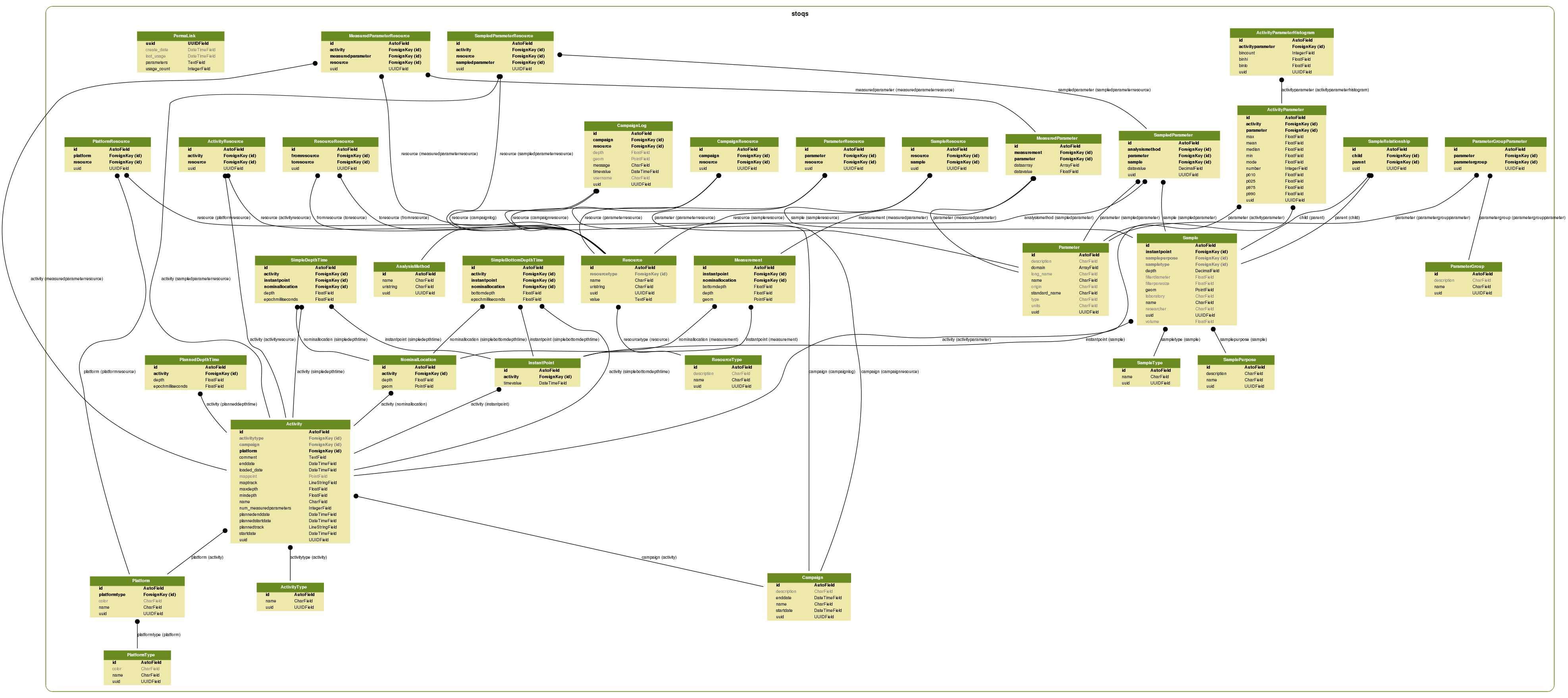
Define our database and a GeoDjango query set for data within 0.1 km of the MARS site.
db = 'stoqs_rovctd_mb'

from django.contrib.gis.geos import fromstr
from django.contrib.gis.measure import D

mars = fromstr('POINT(-122.18681000 36.71137000)')
near_mars = Measurement.objects.using(db).filter(geom__distance_lt=(mars, D(km=.1)))
Count all of the the ROV dives whose Measurements are near MARS
mars_dives = Activity.objects.using(db).filter(instantpoint__measurement=near_mars
                                              ).distinct()
print mars_dives.count()
121
Near surface ROV location data is notoriously noisy (because of fundamental inaccuracies of USBL navigation systems). Let's remove near surface Measurment values from our selection. Count all of the dives near MARS and whose Measurments are deeper than 800 m.
deep_mars_dives = Activity.objects.using(db
                                        ).filter(instantpoint__measurement=near_mars,
                                                 instantpoint__measurement__depth__gt=800
                                                ).distinct()
print deep_mars_dives.count()
99
Let's plot the measurement points of dives on a map of Monterey Bay to confirm that the selection is in the right spot.
%%time
%matplotlib inline
import pylab as plt
from mpl_toolkits.basemap import Basemap

m = Basemap(projection='cyl', resolution='l',
            llcrnrlon=-122.7, llcrnrlat=36.5,
            urcrnrlon=-121.7, urcrnrlat=37.0)
m.arcgisimage(server='http://services.arcgisonline.com/ArcGIS', service='Ocean_Basemap')

for dive in deep_mars_dives:
    points = Measurement.objects.using(db).filter(instantpoint__activity=dive,
                                                  instantpoint__measurement__depth__gt=800
                                                 ).values_list('geom', flat=True)
    m.scatter(
        [geom.x for geom in points],
        [geom.y for geom in points])
CPU times: user 3.57 s, sys: 68 ms, total: 3.63 s
Wall time: 10.1 s

(The major cluster is around the MARS site, but there are a few spurious navigation points even for the deep dive data.)
Let's plot CTD profiles for these dives.
%%time
# A Python dictionary comprehension for all the Parameters and axis labels we want to plot
parms = {p.name: '{} ({})'.format(p.long_name, p.units) for
                 p in Parameter.objects.using(db).filter(name__in=
                        ('t', 's', 'o2', 'sigmat', 'spice', 'light'))}

plt.rcParams['figure.figsize'] = (18.0, 8.0)
fig, ax = plt.subplots(1, len(parms), sharey=True)
ax[0].invert_yaxis()
ax[0].set_ylabel('Depth (m)')

dive_names = []
for dive in deep_mars_dives.order_by('startdate'):
    dive_names.append(dive.name)
    # Use select_related() to improve query performance for the depth lookup
    # Need to also order by time
    mps = MeasuredParameter.objects.using(db
                                ).filter(measurement__instantpoint__activity=dive
                                ).select_related('measurement'
                                ).order_by('measurement__instantpoint__timevalue')
    depth = [mp.measurement.depth for mp in mps.filter(parameter__name='t')]
    for i, (p, label) in enumerate(parms.iteritems()):
        ax[i].set_xlabel(label)
        try:
            ax[i].plot(mps.filter(parameter__name=p).values_list(
                    'datavalue', flat=True), depth)
        except ValueError:
            pass

from IPython.display import display, HTML
display(HTML('<p>All dives at MARS site: ' + ' '.join(dive_names) + '<p>'))
All dives at MARS site: V2439 T660 V2650 V2651 V2780 V2821 V2822 V2825 V2851 V2855 V2893 V2894 T1035 V2895 V3011 V3016 V3127 V3132 V3136 V3170 V3177 V3178 V3179 V3251 V3252 V3280 V3294 V3297 V3328 V3341 V3343 V3344 V3350 D19 V3368 V3373 V3400 V3402 V3424 V3425 V3444 V3472 V3482 V3509 V3517 D114 D118 V3545 V3556 V3561 V3565 V3566 V3569 V3572 V3573 V3576 V3577 V3585 D192 V3586 V3596 V3598 V3601 D222 V3623 V3624 V3625 V3631 V3635 V3636 D248 V3638 D291 D296 D298 D299 V3648 V3654 V3655 D302 V3658 V3659 V3660 V3662 V3665 D320 V3667 D332 D425 D426 D427 V3675 V3689 V3751 V3758 D578 D703 V3831 V3852
CPU times: user 8.72 s, sys: 182 ms, total: 8.9 s
Wall time: 21.5 s
