Quantization of Signals
This jupyter notebook is part of a collection of notebooks on various topics of Digital Signal Processing. Please direct questions and suggestions to Sascha.Spors@uni-rostock.de.
Characteristic of a Linear Uniform Quantizer
The characteristics of a quantizer depend on the mapping functions $f(\cdot)$, $g(\cdot)$ and the rounding operation $\lfloor \cdot \rfloor$ introduced in the previous section. A linear quantizer bases on linear mapping functions $f(\cdot)$ and $g(\cdot)$. A uniform quantizer splits the mapped input signal into quantization steps of equal size. Quantizers can be described by their nonlinear in-/output characteristic $x_Q[k] = \mathcal{Q} \{ x[k] \}$, where $\mathcal{Q} \{ \cdot \}$ denotes the quantization process. For linear uniform quantization it is common to differentiate between two characteristic curves, the so called mid-tread and mid-rise. Both are introduced in the following.
Mid-Tread Characteristic Curve
The in-/output relation of the mid-tread quantizer is given as
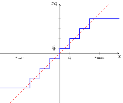
\begin{equation} x_Q[k] = Q \cdot \underbrace{\left\lfloor \frac{x[k]}{Q} + \frac{1}{2} \right\rfloor}_{index} \end{equation}where $Q$ denotes the constant quantization step size and $\lfloor \cdot \rfloor$ the floor function which maps a real number to the largest integer not greater than its argument. Without restricting $x[k]$ in amplitude, the resulting quantization indexes are countable infinite. For a finite number of quantization indexes, the input signal has to be restricted to a minimal/maximal amplitude $x_\text{min} < x[k] < x_\text{max}$ before quantization. The resulting quantization characteristic of a linear uniform mid-tread quantizer is shown below

The term mid-tread is due to the fact that small values $|x[k]| < \frac{Q}{2}$ are mapped to zero.
Example - Mid-tread quantization of a sine signal
The quantization of one period of a sine signal $x[k] = A \cdot \sin[\Omega_0\,k]$ by a mid-tread quantizer is simulated. $A$ denotes the amplitude of the signal, $x_\text{min} = -1$ and $x_\text{max} = 1$ are the smallest and largest output values of the quantizer, respectively.
import numpy as np
import matplotlib.pyplot as plt

A = 1.2  # amplitude of signal
Q = 1 / 10  # quantization stepsize
N = 2000  # number of samples


def uniform_midtread_quantizer(x, Q):
    """Uniform mid-tread quantizer with limiter."""
    # limiter
    x = np.copy(x)
    idx = np.where(np.abs(x) >= 1)
    x[idx] = np.sign(x[idx])
    # linear uniform quantization
    xQ = Q * np.floor(x / Q + 1 / 2)

    return xQ


def plot_signals(x, xQ):
    """Plot continuous, quantized and error signal."""
    e = xQ - x
    plt.figure(figsize=(10, 6))
    plt.plot(x, label=r"signal $x[k]$")
    plt.plot(xQ, label=r"quantized signal $x_Q[k]$")
    plt.plot(e, label=r"quantization error $e[k]$")
    plt.xlabel(r"$k$")
    plt.axis([0, N, -1.1 * A, 1.1 * A])
    plt.legend()
    plt.grid()


# generate signal
x = A * np.sin(2 * np.pi / N * np.arange(N))
# quantize signal
xQ = uniform_midtread_quantizer(x, Q)
# plot signals
plot_signals(x, xQ)
Exercise
- Change the quantization stepsize
Qand the amplitudeAof the signal. Which effect does this have on the quantization error?
Solution: The smaller the quantization step size, the smaller the quantization error is for $|x[k]| < 1$. Note, the quantization error is not bounded for $|x[k]| > 1$ due to the clipping of the signal $x[k]$.
Mid-Rise Characteristic Curve
The in-/output relation of the mid-rise quantizer is given as
\begin{equation} x_Q[k] = Q \cdot \Big( \underbrace{\left\lfloor\frac{ x[k] }{Q}\right\rfloor}_{index} + \frac{1}{2} \Big) \end{equation}where $\lfloor \cdot \rfloor$ denotes the floor function. The quantization characteristic of a linear uniform mid-rise quantizer is illustrated below
The term mid-rise copes for the fact that $x[k] = 0$ is not mapped to zero. Small positive/negative values around zero are mapped to $\pm \frac{Q}{2}$.
Example - Mid-rise quantization of a sine signal
The previous example is now reevaluated using the mid-rise characteristic
A = 1.2  # amplitude of signal
Q = 1 / 10  # quantization stepsize
N = 2000  # number of samples


def uniform_midrise_quantizer(x, Q):
    """Uniform mid-rise quantizer with limiter."""
    # limiter
    x = np.copy(x)
    idx = np.where(np.abs(x) >= 1)
    x[idx] = np.sign(x[idx])
    # linear uniform quantization
    xQ = Q * (np.floor(x / Q) + 0.5)

    return xQ


# generate signal
x = A * np.sin(2 * np.pi / N * np.arange(N))
# quantize signal
xQ = uniform_midrise_quantizer(x, Q)
# plot signals
plot_signals(x, xQ)
Exercise
- What are the differences between the mid-tread and the mid-rise characteristic curves for the given example?
Solution: The mid-tread and the mid-rise quantization of the sine signal differ for signal values smaller than half of the quantization interval. Mid-tread has a representation of $x[k] = 0$ while this is not the case for the mid-rise quantization.
Copyright
This notebook is provided as Open Educational Resource. Feel free to use the notebook for your own purposes. The text is licensed under Creative Commons Attribution 4.0, the code of the IPython examples under the MIT license. Please attribute the work as follows: Sascha Spors, Digital Signal Processing - Lecture notes featuring computational examples.