Quantization of Signals
This jupyter notebook is part of a collection of notebooks on various topics of Digital Signal Processing. Please direct questions and suggestions to Sascha.Spors@uni-rostock.de.
Introduction
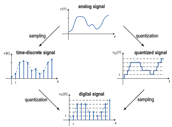
Digital signal processors and general purpose processors can only perform arithmetic operations within a limited number range. So far we considered discrete signals with continuous amplitude values. These cannot be handled by processors in a straightforward manner. Quantization is the process of mapping a continuous amplitude to a countable set of amplitude values. This refers also to the requantization of a signal from a large set of countable amplitude values to a smaller set. Scalar quantization is an instantaneous and memoryless operation. It can be applied to the continuous amplitude signal, also referred to as analog signal or to the (time-)discrete signal. The quantized discrete signal is termed as digital signal. The connections between the different domains are illustrated in the following.
Model of the Quantization Process
In order to discuss the effects of quantizing a continuous amplitude signal, a mathematical model of the quantization process is required. We restrict our considerations to a discrete real-valued signal $x[k]$. The following mapping is used in order to quantize the continuous amplitude signal $x[k]$
\begin{equation} x_Q[k] = g( \; \lfloor \, f(x[k]) \, \rfloor \; ) \end{equation}where $g(\cdot)$ and $f(\cdot)$ denote real-valued mapping functions, and $\lfloor \cdot \rfloor$ a rounding operation. The quantization process can be split into two stages
Forward quantization The mapping $f(x[k])$ maps the signal $x[k]$ such that it is suitable for the rounding operation. This may be a scaling of the signal or a non-linear mapping. The result of the rounding operation is an integer number $\lfloor \, f(x[k]) \, \rfloor \in \mathbb{Z}$, which is termed as quantization index.
Inverse quantization The mapping $g(\cdot)$, maps the quantization index to the quantized value $x_Q[k]$ such that it constitutes an approximation of $x[k]$. This may be a simple scaling or non-linear operation.
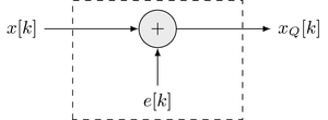
The quantization error (quantization noise) $e[k]$ is defined as
\begin{equation} e[k] = x_Q[k] - x[k] \end{equation}Rearranging yields that the quantization process can be modeled by adding the quantization error to the discrete signal
Example - Quantization of a sine signal
In order to illustrate the introduced model, the quantization of one period of a sine signal is considered
\begin{equation} x[k] = \sin[\Omega_0 k] \end{equation}using
\begin{align} f(x[k]) &= 3 \cdot x[k] \\ i &= \lfloor \, f(x[k]) \, \rfloor \\ g(i) &= \frac{1}{3} \cdot i \end{align}where $\lfloor \cdot \rfloor$ denotes the nearest integer function and $i$ the quantization index. The quantized signal is then given as
\begin{equation} x_Q[k] = \frac{1}{3} \cdot \lfloor \, 3 \cdot \sin[\Omega_0 k] \, \rfloor \end{equation}The discrete signals are not shown by stem plots for ease of illustration.
import numpy as np
import matplotlib.pyplot as plt

N = 1024  # length of signal

# generate signal
x = np.sin(2 * np.pi / N * np.arange(N))
# quantize signal
xi = np.round(3 * x)
xQ = 1 / 3 * xi
e = xQ - x

# plot (quantized) signals
fig, ax1 = plt.subplots(figsize=(10, 4))
ax2 = ax1.twinx()

ax1.plot(x, "r", label=r"signal $x[k]$")
ax1.plot(xQ, "b", label=r"quantized signal $x_Q[k]$")
ax1.plot(e, "g", label=r"quantization error $e[k]$")
ax1.set_xlabel("k")
ax1.set_ylabel(r"$x[k]$, $x_Q[k]$, $e[k]$")
ax1.axis([0, N, -1.2, 1.2])
ax1.legend()

ax2.set_ylim([-3.6, 3.6])
ax2.set_ylabel("quantization index")
ax2.grid()
Exercise
- Investigate the quantization error $e[k]$. Is its amplitude bounded?
- If you would represent the quantization index (shown on the right side) by a binary number, how much bits would you need?
- Try out other rounding operations like
np.floor()andnp.ceil()instead ofnp.round(). What changes?
Solution: It can be concluded from the illustration that the quantization error is bounded as $|e[k]| < \frac{1}{3}$. There are in total 7 quantization indexes needing 3 bits in a binary representation. The properties of the quantization error are different for different rounding operations.
Properties
Without knowledge of the quantization error $e[k]$, the signal $x[k]$ cannot be reconstructed exactly from its quantization index or quantized representation $x_Q[k]$. The quantization error $e[k]$ itself depends on the signal $x[k]$. Therefore, quantization is in general an irreversible process. The mapping from $x[k]$ to $x_Q[k]$ is furthermore non-linear, since the superposition principle does not hold in general. Summarizing, quantization is an inherently irreversible and non-linear process. It potentially removes information from the signal.
Applications
Quantization has widespread applications in Digital Signal Processing. For instance
- Analog-to-Digital conversion
- Lossy compression of signals (speech, music, video, ...)
- Storage and transmission (Pulse-Code Modulation, ...)
Copyright
This notebook is provided as Open Educational Resource. Feel free to use the notebook for your own purposes. The text is licensed under Creative Commons Attribution 4.0, the code of the IPython examples under the MIT license. Please attribute the work as follows: Sascha Spors, Digital Signal Processing - Lecture notes featuring computational examples.