Make me look good. Click on the cell below and press Ctrl+Enter.
from IPython.core.display import HTML
HTML(open('css/custom.css', 'r').read())
SM286D · Introduction to Applied Mathematics with Python · Spring 2020 · Uhan
Lesson 12.
Graph theory with Python
This lesson...
Introduction to graph theory
Using NetworkX to compute measures of centrality/influence
- Degree centrality
- Closeness centrality
- Betweenness centrality
Introduction to graph theory
Graphs model how various entities are connected.
Graphs have numerous and diverse applications throughout operations research, including in utility planning, job scheduling, task assignment, and modeling networks.
Graphs are a central focus of SM342, our class in discrete mathematics (a math or breadth elective in the Operations Research major).
A graph $G = (V,E)$ consists of
- a set of vertices $V$ (also called nodes), and
- a set $E$ of pairs of vertices.
In an undirected graph, each pair $(v_1, v_2) \in E$ is an edge with endpoints $v_1$ and $v_2$.
- For edges, direction doesn't matter: the edges $(v_1,v_2)$ and $(v_2,v_1)$ are the same.
- We use line segments to draw edges.
In a directed graph, each pair $(v_1, v_2) \in E$ is an arc that starts at $v_1$ and ends at $v_2$.
- For arcs, direction matters: the arcs $(v_1, v_2)$ and $(v_2, v_1)$ are NOT the same.
- We use arrows to draw arcs.
Figure 1 shows an example of an undirected graph $G$.
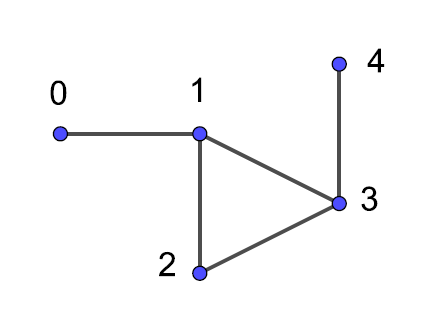
Example. Is $(0, 1)$ an edge of $G$? Is $(0, 2)$ an edge of $G$?
Write your notes here. Double-click to edit.
- For this lesson, we will focus on undirected graphs — we will simply call them graphs.
- We often describe a graph by its adjacency matrix $A$: a square matrix with one row and one column for each node, where
- The adjacency matrix for $G$ in Figure 1 is
- The degree of a node $v$ is the number of edges that contain $v$.
- In Figure 1, you can see the degree of a node by seeing how many edges come out of it.
Example. What is the degree of node 3 in graph $G$ in Figure 1?
Write your notes here. Double-click to edit.
A path is a sequence of nodes $(v_1,v_2,v_3,\ldots,v_n)$ such that subsequent nodes $(v_i,v_{i+1})$ form an edge in $G$.
The length of a path is the number of edges it contains.
Example. Consider the graph $G$ in Figure 1. Give an example of a path from node 0 to node 4. What is its length? What is the shortest path from node 0 to node 4?
Write your notes here. Double-click to edit.
Using NetworkX to compute measures of centrality/influence
In today's lesson and Project 5, we will be using Python to compute measures of centrality/influence in social networks.
Consider the following example.
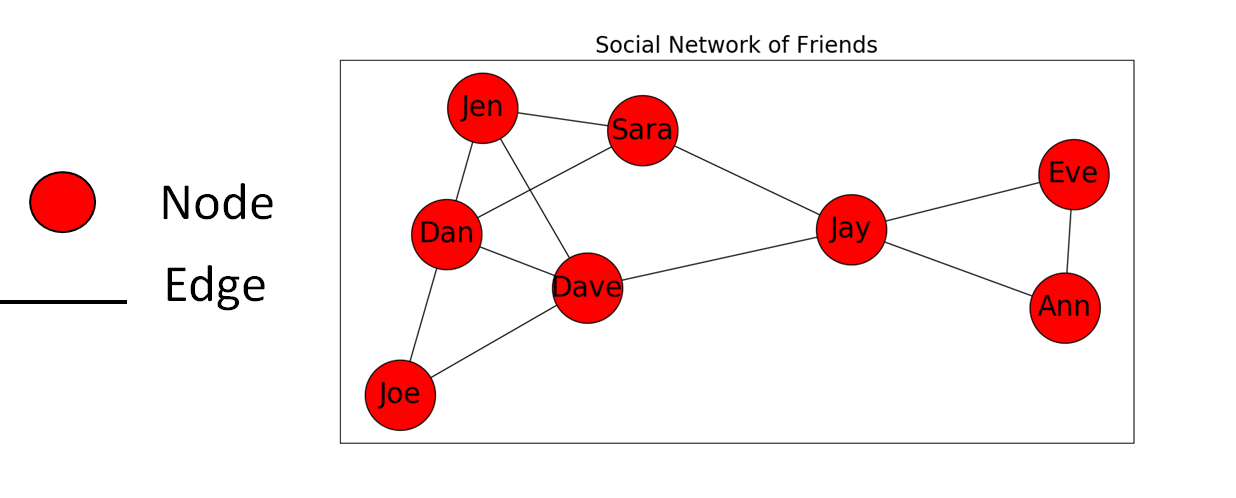
Example. Suppose Ann, Dan, Dave, Eve, Jay, Jen, Joe, and Sara are all on Facebook. Ann is friends with Eve and Jay; Dan is friends with Dave, Jen, Joe, and Sara; Dave is friends with Jay, Joe, and Dan; Eve is friends with Ann and Jay; Jay is friends with Ann, Eve, Dave, and Sara; Jen is friends with Dan, Dave, and Sara; Joe is friends with Dan and Dave; and Sara is friends with Dan, Jay, and Jen.
This is a lot of words to explain the connections between these individuals.
It might be better to illustrate their relationships with a graph. See Figure 2 below.
NetworkX is a Python package that lets us work with graphs.
Let's start with importing
networkx:
import networkx as nx
- Next we define an empty graph
G, followed by the list of nodes and edges:
# Define an empty graph
G = nx.Graph()

# Define the list of nodes
nodes = ['Ann', 'Dan', 'Dave', 'Eve', 'Jay', 'Jen', 'Joe', 'Sara']

# Define the list of edges
# Note that each edge is a list
edges = [['Jay', 'Dave'], ['Sara', 'Dan'], ['Dan', 'Jen'], ['Eve', 'Ann'],
        ['Sara', 'Jen'], ['Jay', 'Ann'], ['Joe', 'Dave'], ['Jay', 'Eve'],
        ['Jen', 'Dave'], ['Jay', 'Sara'], ['Joe', 'Dan'], ['Dan', 'Dave']]
- We can add
nodesandedgesto the graphGlike this:
# Add nodes to G
G.add_nodes_from(nodes)

# Add edges to G
G.add_edges_from(edges)
- Now that we've defined the network, a natural question to ask is:
- There are many ways to measure this. We will discuss three of them here.
Degree centrality
Recall that the degree of a node is the number of edges containing that node.
Figure 3 below shows our social network example with the degree of each node listed next to it.

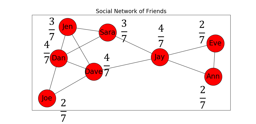
The degree centrality of a node is defined as the node's degree divided by the maximum possible degree.
The maximum possible degree is given by $N-1$, where $N$ is the total number of nodes in the graph.
- For our example, the maximum possible degree is 7.
Figure 4 below shows our social network with the degree centrality of each node listed next to it.
- To compute the degree centrality of each node in a graph using NetworkX, we can do this:
# Compute degree centrality for each node
degree_centrality = nx.degree_centrality(G)

# Check our work
print(degree_centrality)
{'Ann': 0.2857142857142857, 'Dan': 0.5714285714285714, 'Dave': 0.5714285714285714, 'Eve': 0.2857142857142857, 'Jay': 0.5714285714285714, 'Jen': 0.42857142857142855, 'Joe': 0.2857142857142857, 'Sara': 0.42857142857142855}
We see that
nx.degree_centrality()returns a dictionary.Let's print this information nicely:
# Print degree centrality for each node
for key, value in degree_centrality.items():
    print(f'{key} has degree centrality {value:.3f}.')
Ann has degree centrality 0.286.
Dan has degree centrality 0.571.
Dave has degree centrality 0.571.
Eve has degree centrality 0.286.
Jay has degree centrality 0.571.
Jen has degree centrality 0.429.
Joe has degree centrality 0.286.
Sara has degree centrality 0.429.
Closeness centrality
Another way to measure the centrality/influence of a member of the network is closeness centrality.
In order to define closeness centrality, we begin by looking at the shortest path distance between two nodes.
The shortest path distance between two nodes is simply the length of a shortest path between the two nodes.
Let's use Jay as the starting node, and find the shortest path from Jay to all the other nodes in the graph.
- This process is illustrated in Figure 5 below.
Next we find the sum of the shortest path distances from Jay to all the other nodes:
\begin{equation*} 1 + 1 + 1 + 2 + 2 + 2 + 1 = 10 \end{equation*}
The closeness $c$ of a node measures how close it is to every other node.
The closeness of the node Jay is given by
\begin{equation*} c(\text{Jay}) = \frac{1}{\sum_{i} d(i,\text{Jay})} = \frac{1}{10} \end{equation*}
where $d(i,\rm{Jay})$ is the shortest path distance from node $i$ to node $\rm{Jay}$.
The closeness centrality of the node Jay is
\begin{equation*} C(\text{Jay}) = (N-1)c(\text{Jay}) \end{equation*}
where $N$ is the total number of nodes in the graph.
For our example, the closeness centrality of node Jay is
\begin{equation*} C(\text{Jay}) = (N - 1) c(\text{Jay}) = (8-1) \frac{1}{10} = \frac{7}{10} \end{equation*}
Figure 6 below shows our social network example with the closeness centrality of each node listed next to it.
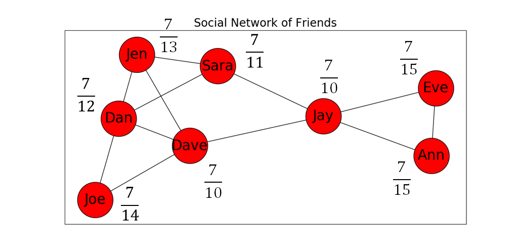
- To compute the closeness centrality of each node in a graph using NetworkX, we can do this:
# Compute closeness centrality for each node
closeness_centrality = nx.closeness_centrality(G)

# Check our work
print(closeness_centrality)
{'Ann': 0.4666666666666667, 'Dan': 0.5833333333333334, 'Dave': 0.7, 'Eve': 0.4666666666666667, 'Jay': 0.7, 'Jen': 0.5384615384615384, 'Joe': 0.5, 'Sara': 0.6363636363636364}
Like
nx.degree_centrality(),nx.closeness_centrality()also returns a dictionary.Let's print this information nicely:
# Print closeness centrality for each node
for key, value in closeness_centrality.items():
    print(f'{key} has closeness centrality {value:.3f}.')
Ann has closeness centrality 0.467.
Dan has closeness centrality 0.583.
Dave has closeness centrality 0.700.
Eve has closeness centrality 0.467.
Jay has closeness centrality 0.700.
Jen has closeness centrality 0.538.
Joe has closeness centrality 0.500.
Sara has closeness centrality 0.636.
Betweenness centrality
Yet another way to measure the centrality/influence of a member of the network is betweenness centrality.
The betweenness centrality of a node measures how often it is on the shortest path between two other nodes.
This is illustrated in Figure 7 below where we are looking at shortest paths from Dave to other nodes.
- We see that Jay is on the shortest path from Dave to Eve and Dave to Sara, but Jay is not on the shortest path from Dave to Dan.

- To compute the betweenness centrality of each node in a graph using NetworkX, we can do this:
# Compute betweenness centrality for each node
betweenness_centrality = nx.betweenness_centrality(G)

# Check our work
print(betweenness_centrality)
{'Ann': 0.0, 'Dan': 0.08730158730158728, 'Dave': 0.30952380952380953, 'Eve': 0.0, 'Jay': 0.492063492063492, 'Jen': 0.015873015873015872, 'Joe': 0.0, 'Sara': 0.14285714285714285}
Yup,
nx.betweenness_centrality()also returns a dictionary.Let's print this information nicely:
# Print betweenness centrality for each node
for key, value in betweenness_centrality.items():
    print(f'{key} has betweenness centrality {value:.3f}.')
Ann has betweenness centrality 0.000.
Dan has betweenness centrality 0.087.
Dave has betweenness centrality 0.310.
Eve has betweenness centrality 0.000.
Jay has betweenness centrality 0.492.
Jen has betweenness centrality 0.016.
Joe has betweenness centrality 0.000.
Sara has betweenness centrality 0.143.
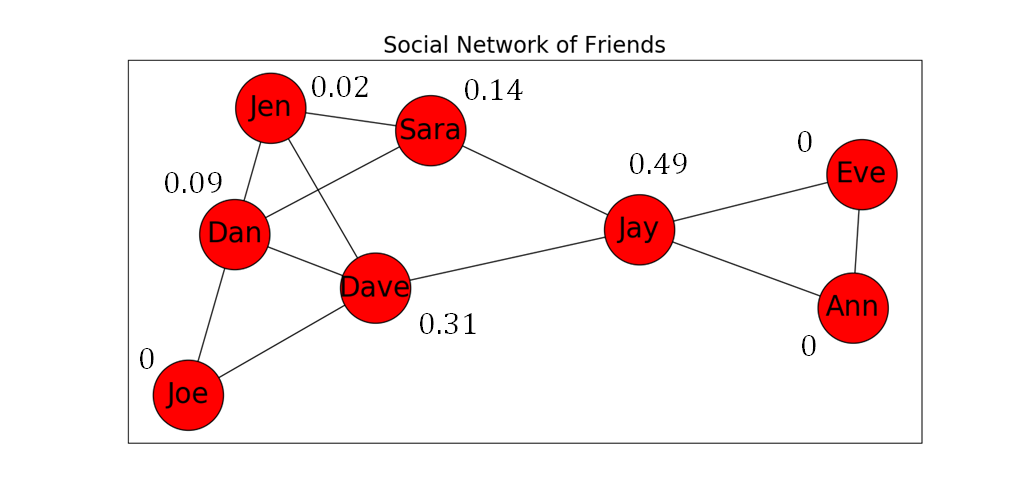
- Figure 8 below shows our social network example with the betweenness centrality of each node listed next to it.
So... who is the most central/influential of the group?
As usual, the answer is, "it depends".
In particular, it depends on which measure you want to use.
The table below summarizes the results from the three measures we explored above.
| Degree Centrality | Closeness Centrality | Betweenness Centrality |
|---|---|---|
| 1. Dan - 0.571 | 1. Dave - 0.700 | 1. Jay - 0.492 |
| 2. Dave - 0.571 | 2. Jay - 0.700 | 2. Dave - 0.310 |
| 3. Jay - 0.571 | 3. Sara - 0.636 | 3. Sara - 0.143 |
Classwork
Problem 1. In the code below, we first define the adjacency matrix of a graph with NumPy. Note the way that we filled in a different row of $A$ on each of lines 6 through 10. For example, on line 7 we filled row 1 by setting $A_{10} = A_{12} = A_{13} = 1$.
On line 13, we use the adjacency matrix $A$ to define the graph $G$. Note that this is different from how we defined a graph in the lesson above. We get a list of the nodes of $G$ on line 14 and a list of the edges of $G$ on line 15.
import numpy as np
import networkx as nx

# Define adjacency matrix
A = np.zeros([5,5])
A[0, [1]] = 1
A[1, [0, 2, 3]] = 1
A[2, [1, 3]] = 1
A[3, [1, 2, 4]] = 1
A[4, [3]] = 1

# Define graph using NetworkX
G = nx.Graph(A)
nodes_list = list(G.nodes)
edges_list = list(G.edges)
Print the lists of nodes and edges to the screen. Make sure you understand why they look the way they do.
print(f'Nodes: {nodes_list}')
print(f'Edges: {edges_list}')
Nodes: [0, 1, 2, 3, 4]
Edges: [(0, 1), (1, 2), (1, 3), (2, 3), (3, 4)]
Problem 2. You can draw a graph G with nx.draw_networkx(G). Use this to draw the graph G defined in Problem 1. Do you see what you expected?
You may need to import the matplotlib.pyplot package as plt to get the drawing to work.
Take a look at the documentation if you need to. Try calling nx.draw_networkx() with the keyword arguments with_labels=True and font_color='w'.
import matplotlib.pyplot as plt
nx.draw_networkx(G, with_labels=True, font_color='w')
Problem 3. The graph G you defined in Problem 1 has a variety of methods and attributes. For example, the attribute G.nodes is a list-like object that contains all the nodes of G. As another example, the method G.degree() returns a data structure that contains the degree for each vertex: in particular, you can access the degree of vertex $j$ with G.degree()[j]. Use a for loop to print a sentence like
The degree of vertex 0 is 1.
for each vertex in G.
for n in G.nodes:
    print(f'The degree of vertex {n} is {G.degree()[n]}.')
The degree of vertex 0 is 1.
The degree of vertex 1 is 3.
The degree of vertex 2 is 2.
The degree of vertex 3 is 3.
The degree of vertex 4 is 1.
Problem 4.
You can find the vertices connected to vertex v in graph G with G.neighbors(v). However, it returns a strange (dict_keyiterator) object. You can call list() on the result of G.neighbors(v) to turn it into something readable.
Print the list of neighbors of vertex 2.
two_neighbors = list(G.neighbors(2))
print(f'The neighbors of node 2 are the elements of the list {two_neighbors}.')
The neighbors of node 2 are the elements of the list [1, 3].
Problem 5. You can find the length of a shortest path from node 0 to node 4 with
nx.shortest_path_length(G, source=0, target=4)
In today's lesson, we called this the shortest path distance between node 0 and node 4. The method nx.shortest_path() produces the path itself.
Modify the code in Problem 1 to construct the adjacency matrix B for a new graph with edges (0, 1), (0, 3), (1, 2), (2, 3), and (3, 4). Let H be the graph with adjacency matrix B. Find the shortest path length between 1 and 4. Use the nx.all_shortest_paths() method to find all the shortest paths from node 1 to node 4 in H. Read the NetworkX documentation if you're not sure how to use nx.all_shortest_paths().
# Define adjacency matrix
B = np.zeros([5,5])
B[0, [1, 3]] = 1
B[1, [0, 2]] = 1
B[2, [1, 3]] = 1
B[3, [0, 2, 4]] = 1
B[4, [3]] = 1

# Define graph using adjacency matrix
H = nx.Graph(B)

# Compute shortest path information
print(f'The shortest path distance from node 1 to node 4 is {nx.shortest_path_length(H, source=1, target=4)}')
print(f'The shortest paths from node 1 to node 4 are: ')
for i in nx.all_shortest_paths(H, source=1, target=4):
    print(i)
The shortest path distance from node 1 to node 4 is 3
The shortest paths from node 1 to node 4 are:
[1, 0, 3, 4]
[1, 2, 3, 4]
Problem 6.
The graph H from the last problem is really a graph of friendships among five people. Create a names dictionary that maps node numbers as keys to names as values as follows: Suzie (node 0), Tom (node 1), Jamal (node 2), Heather (node 3), and Nitish (node 4).
In H, we see that Suzie is friends (separately) with Tom and Heather. Print the two shortest paths from Tom to Nitish, using names rather than node numbers. Do this without hard coding your answer (i.e. refer to the names dictionary rather than writing names directly in your code). One of your paths should be:
Tom - Jamal - Heather - Nitish
# Define dictionary that maps node numbers to names
names = {0: 'Suzie', 1: 'Tom', 2: 'Jamal', 3: 'Heather', 4: 'Nitish'}

# Print all shortest paths from Tom to Nitish,
# using names rather than node numbers
print('The shorest paths are: ')
for path in nx.all_shortest_paths(H, source=1, target=4):

    # Create list of names corresponding to path
    # I'm using a list comprehension here, but
    # you can also use a for loop with .append()
    path_names = [names[n] for n in path]

    # Print the list of names, using .join() to format them nicely
    # See Problem 1 from Lesson 10 for more information about .join()
    print(' - '.join(path_names))
The shorest paths are:
Tom - Suzie - Heather - Nitish
Tom - Jamal - Heather - Nitish
Bonus classwork
The following problems are included as bonus material. Work on them only after completing the problems above.
Problem 7 (Directed graphs). Directed graphs are used to model many different situations in operations research. There is a popular OR textbook, Network Flows (by Ravindra K. Ahuja, Thomas L. Magnanti, and James B. Orlin), devoted to the topic and USNA often offers an elective course in this area.
Network flow problems are defined on directed graphs $(V, E)$: the set $E$ consists of arcs $(v_1, v_2)$ that allow flow from vertex $v_1$ to vertex $v_2$. Each vertex has an associated supply or demand, and each edge has an associated capacity and cost.
One type of network flow problem is the maximum flow of minimum cost problem. In this problem, we want to move as much flow along edges from a source vertex to a destination vertex, leaving nothing behind at any other vertex, while respecting the capacity constraints on the edges, and at minimum cost. The decision variables in this problem determine how much to flow along each edge of the network.
The code below solves a maximum flow of minimum cost problem using NetworkX on a directed graph (note the use of DiGraph()) where vertex 1 is the source and vertex 7 is the destination. On paper, draw a picture of the network, and label each edge with capacity/cost/flow, where flow comes from the solution to the problem.
# Define empty directed graph
G = nx.DiGraph()

# Add edges to directed graph
# Note that NetworkX will add the corresponding nodes automatically
# Also note that some edges do not have 'capacity' defined:
# read the documentation to understand what this means.
G.add_edges_from([(1, 2, {'capacity': 12, 'weight': 4}),
                  (1, 3, {'capacity': 20, 'weight': 6}),
                  (2, 3, {'capacity': 6, 'weight': -3}),
                  (2, 6, {'capacity': 14, 'weight': 1}),
                  (3, 4, {'weight': 9}),
                  (3, 5, {'capacity': 10, 'weight': 5}),
                  (4, 2, {'capacity': 19, 'weight': 13}),
                  (4, 5, {'capacity': 4, 'weight': 0}),
                  (5, 7, {'capacity': 28, 'weight': 2}),
                  (6, 5, {'capacity': 11, 'weight': 1}),
                  (6, 7, {'weight': 8}),
                  (7, 4, {'capacity': 6, 'weight': 6})])

# Find the max flow of min cost from vertex 1 to vertex 7
# Read the documentation to understand the structure of the
# dictionary that nx.max_flow_min_cost returns.
min_cost_flow = nx.max_flow_min_cost(G, s=1, t=7)
print(min_cost_flow)

# Compute the cost of the max flow of min cost
min_cost = nx.cost_of_flow(G, min_cost_flow)
print(min_cost)
{1: {2: 12, 3: 16}, 2: {3: 0, 6: 14}, 3: {4: 6, 5: 10}, 6: {5: 11, 7: 3}, 4: {2: 2, 5: 4}, 5: {7: 25}, 7: {4: 0}}
373

Problem 8 (Eulerian graphs). A path in an undirected graph $G$ is called Eulerian if it uses all of the edges of $G$ precisely once. A path where the initial vertex and the last vertex are the same is called a cycle or a circuit. A graph $G$ that has an Eulerian cycle (an Eulerian path that is also a cycle) is called an Eulerian graph, named after Leonhard Euler (look up the Königsberg Bridge Problem if you are curious about how such graphs first appeared).
Define a graph $P$ with six vertices 0, 1, 2, 3, 4 and 5 and edges (0, 1), (0, 3), (1, 2), (2, 3), (3, 4), (3, 5), (4, 5). Draw $P$ using NetworkX. Then convince yourself that $P$ is Eulerian.
The code
list(nx.eulerian_circuit(G))
produces an Eulerian cycle for a graph G if one exists. Use this code to check your work. Find the degree of each vertex in $P$. The degrees all share a common property; can you guess what it is? Make your guess and then check out the cell below for a fun fact about Eulerian graphs.
# Define adjacency matrix of P
C = np.zeros([6,6])
C[0, [1, 3]] = 1
C[1, [0, 2]] = 1
C[2, [1, 3]] = 1
C[3, [0, 2, 4, 5]] = 1
C[4, [3, 5]] = 1
C[5, [3, 4]] = 1

# Define graph P based on adjacency matrix
P = nx.Graph(C)

# Draw the graph
nx.draw_networkx(P, with_labels=True, font_color='w')

# Find an Eulerian circuit and print the output
print(f'Eulerian circuit: {list(nx.eulerian_circuit(P))}')

# Print the degree of every vertex
for i in P.nodes:
    print(f'Degree of vertex {i}: {P.degree()[i]}')

print('All the degrees are even!')
Eulerian circuit: [(0, 3), (3, 5), (5, 4), (4, 3), (3, 2), (2, 1), (1, 0)]
Degree of vertex 0: 2
Degree of vertex 1: 2
Degree of vertex 2: 2
Degree of vertex 3: 4
Degree of vertex 4: 2
Degree of vertex 5: 2
All the degrees are even!

It turns out that every vertex in an Eulerian graph has even degree. In fact, if the graph is connected (any two vertices can be connected by a path) and every vertex has even degree, then the graph is also Eulerian!
Problem 9 (Planarity). A (undirected) graph is called planar if it can be drawn in the plane without edges crossing (you are allowed to draw the graph edges as curved lines if you like). All the graphs we've seen so far have been planar graphs.
Two non-planar graphs are $K_{5}$ and $K_{3,3}$. The graph $K_{5}$ is called the complete graph on 5 vertices. It has ... wait for it ... five vertices. And it is complete in the sense that every possible edge is in the graph: every pair of vertices is connected by an edge.
The graph $K_{3,3}$ is an example of a complete bipartite graph. Such graphs have two kinds of vertices (call them blue and gold) and all possible edges between blue and gold vertices are present while no edges between vertices of the same color are present. The graph $K_{3,3}$ has 3 vertices of each color.
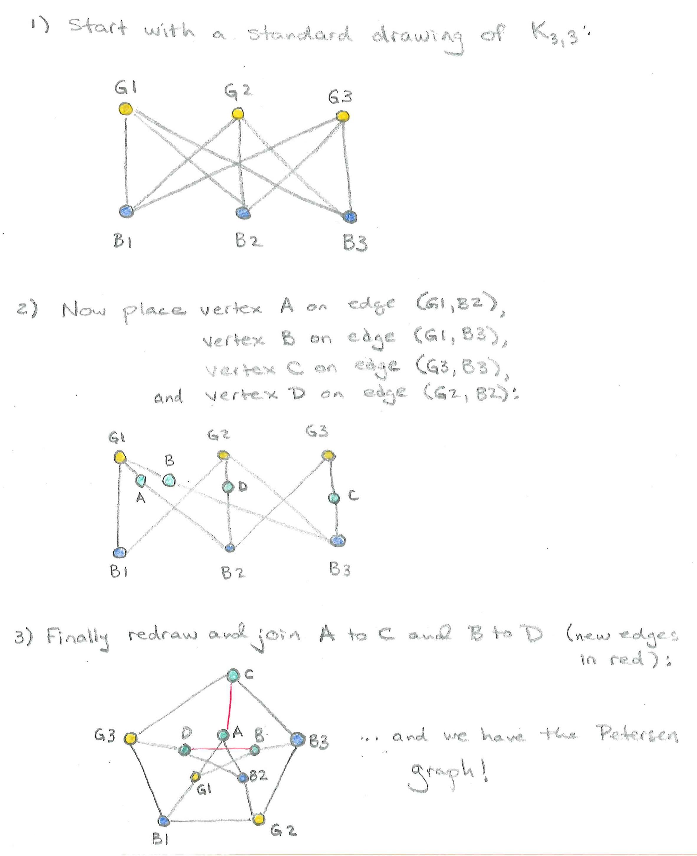
In fact, in a precise sense, these are the only examples of non-planar graphs. It turns out that every other non-planar graph can be obtained from $K_5$ or $K_{3,3}$ by a combination of actions: adding edges between existing vertices, subdividing an existing edge by inserting a vertex on the edge, or adding new vertices. The Petersen graph is the graph pictured in Figure 9.
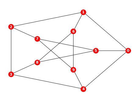
It is a counterexample to many natural conjectures in graph theory. In the code below, we define the Petersen graph in NetworkX using nx.petersen_graph(), and draw the graph.
# Define Petersen graph in NetworkX
G = nx.petersen_graph()

# Draw the Petersen graph
nx.draw_shell(G, nlist=[range(5, 10), range(5)], with_labels=True, font_weight='bold', font_color='w')

Use the code below to learn whether the Petersen graph is planar or not.
Note. You may need to update to the latest version of NetworkX to use
nx.check_planarity(). To do that, go to the Anaconda Prompt (search in the Windows Start Menu) and then typepip install networkx --upgradeYou'll need to restart the kernel in Jupyter in order to access the new version of the package once it is installed.
# Check for planarity
nx.check_planarity(G)
(False, None)
On paper, can you build the Petersen graph from $K_{3,3}$ using the actions described above?