Harmonic Magnetic Dipole Sounding over a Sphere
In this notebook, we will simulate an FDEM sounding over a conductive sphere. A cylindrical mesh and the SimPEG Electromanetics module is used to perform the simulation.
For more on SimPEG and SimPEG.EM see:
- (Cockett et al., 2015): SimPEG: An open source framework for simulation and gradient based parameter estimation in geophysical applications
- (Heagy et al., 2016): A framework for simulation and inversion in electromagnetics
Setup
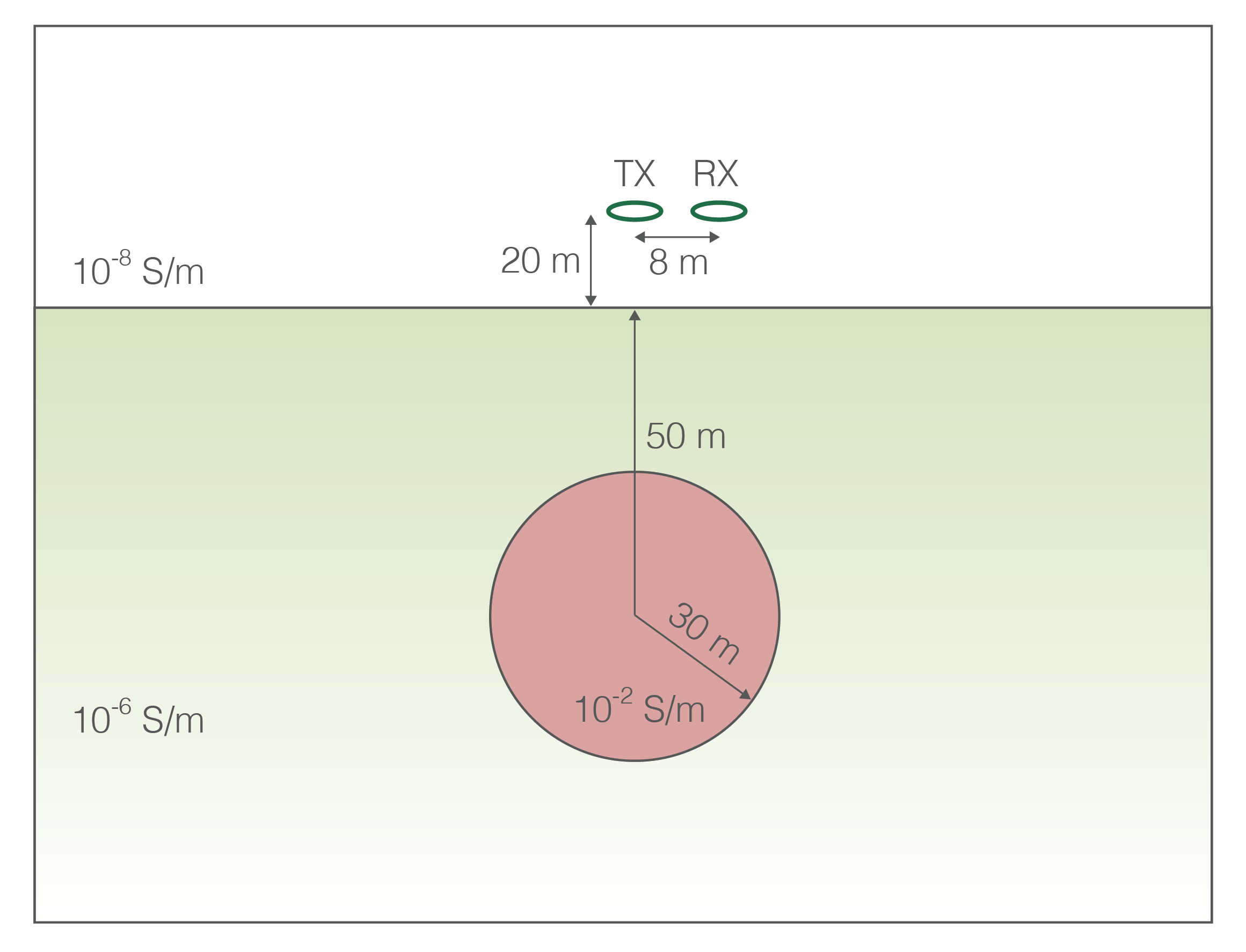
An inductive loop transmitter is centered over an electrically conductive sphere (radius 30m). The transmitter is 20m above the surface, and the center of the sphere is 50m below the surface. A coil receiver is offset by 8m horizontally from the transmitter.
Getting Started: Package Imports
NumPy, SciPy and Matplotlib are core Python packages that can be installed when you install python with a distribution such as Anaconda.
SimPEG is a Simulation and Inversion package for geophysics.
If you would like to set up and run SimPEG on your machine, see http://simpeg.xyz and http://tutorials.simpeg.xyz
# Basic python packages
import numpy as np
import matplotlib.pyplot as plt
from scipy.constants import mu_0

# Modules of SimPEG we will use for forward modelling
from SimPEG import Mesh, Utils, Maps
from SimPEG.EM import FDEM
from SimPEG import SolverLU as Solver

# Set a nice colormap!
plt.set_cmap(plt.get_cmap('viridis'))

%matplotlib inline
Model Parameters
We define a
- resistive halfspace and
- conductive sphere
- radius of 30m
- center is 50m below the surface
# electrical conductivities in S/m
sig_halfspace = 1e-6
sig_sphere = 1e-2
sig_air = 1e-8
# depth to center, radius in m
sphere_z = -50.
sphere_radius = 30.
Survey Parameters
- Transmitter and receiver 20m above the surface
- Receiver offset from transmitter by 8m horizontally
- 25 frequencies, logaritmically between $10^3$ Hz and $10^6$ Hz
boom_height = 20.
rx_offset = 8.
freqs = np.logspace(3, 6, 25)

# source and receiver location in 3D space
src_loc = np.r_[0., 0., boom_height]
rx_loc = np.atleast_2d(np.r_[rx_offset, 0., boom_height])
# print the min and max skin depths to make sure mesh is fine enough and
# extends far enough

def skin_depth(sigma, f):
    return 500./np.sqrt(sigma * f)

print(
    'Minimum skin depth (in sphere): {:.2e} m '.format(skin_depth(sig_sphere, freqs.max()))
)
print(
    'Maximum skin depth (in background): {:.2e} m '.format(skin_depth(sig_halfspace, freqs.min()))
)
Minimum skin depth (in sphere): 5.00e+00 m
Maximum skin depth (in background): 1.58e+04 m
Mesh
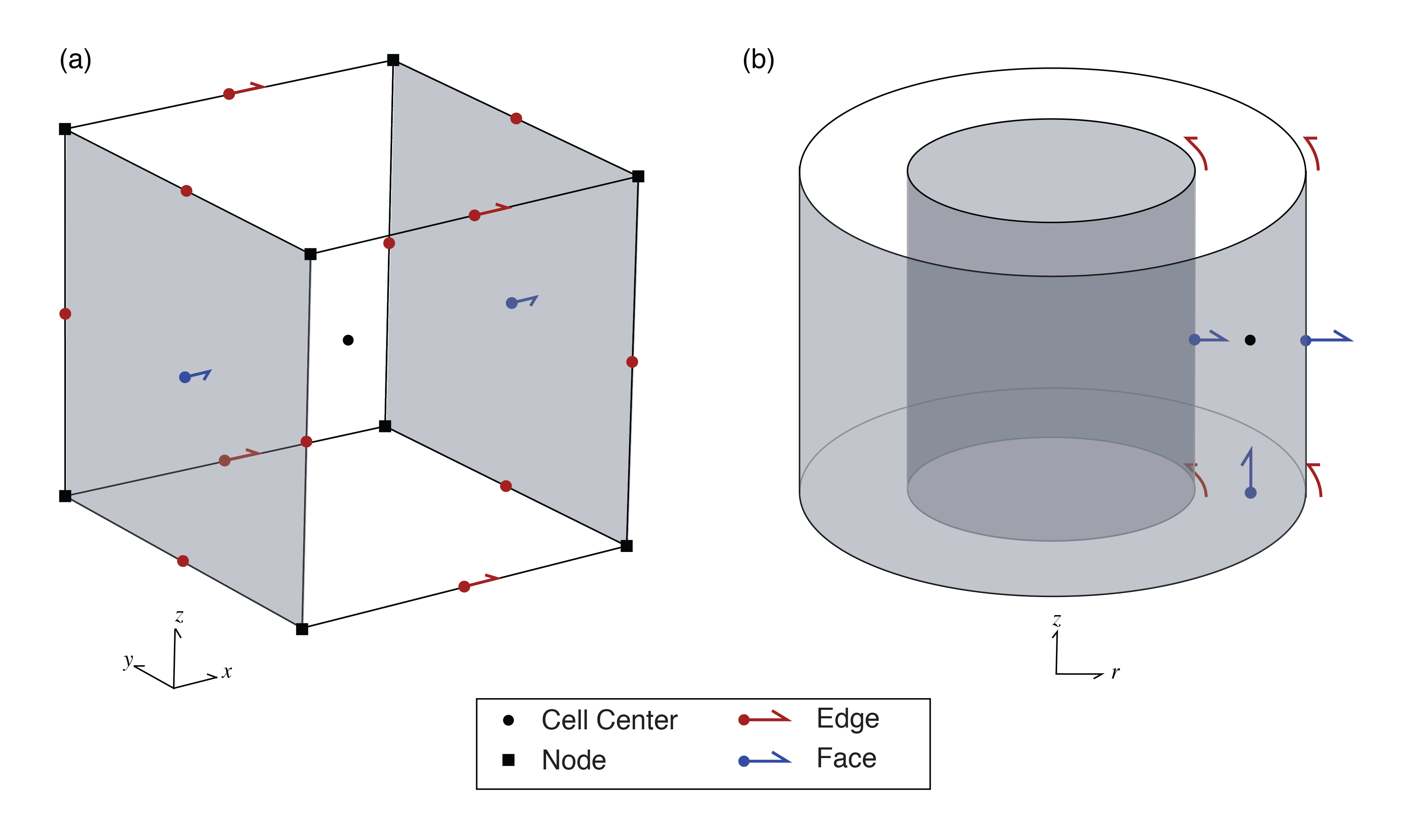
Here, we define a cylindrically symmetric tensor mesh.
The figure below shows a cell in a cartesian mesh (a) and a cylindrically symmetric mesh (b). Note that edges are rotational and faces are radial and vertical in the cylindrically symmetric mesh.
Mesh Parameters
For the mesh, we will use a cylindrically symmetric tensor mesh. To construct a tensor mesh, all that is needed is a vector of cell widths in the x and z-directions. We will define a core mesh region of uniform cell widths and a padding region where the cell widths expand "to infinity".
# x-direction
csx = 2  # core mesh cell width in the x-direction
ncx = np.ceil(1.2*sphere_radius/csx)  # number of core x-cells (uniform mesh slightly beyond sphere radius)
npadx = 30  # number of x padding cells

# z-direction
csz = 1  # core mesh cell width in the z-direction
ncz = np.ceil(1.2*(boom_height - (sphere_z-sphere_radius))/csz) # number of core z-cells (uniform cells slightly below bottom of sphere)
npadz = 32  # number of z padding cells

# padding factor (expand cells to infinity)
pf = 1.3
# cell spacings in the x and z directions
hx = Utils.meshTensor([(csx, ncx), (csx, npadx, pf)])
hz = Utils.meshTensor([(csz, npadz, -pf), (csz, ncz), (csz, npadz, pf)])

# define a SimPEG mesh
mesh = Mesh.CylMesh([hx, 1, hz], x0 = np.r_[0.,0., -hz.sum()/2.-boom_height])
Plot the mesh
Below, we plot the mesh. The cyl mesh is rotated around x=0. Ensure that each dimension extends beyond the maximum skin depth.
Zoom in by changing the xlim and zlim.
# X and Z limits we want to plot to. Try changing them to see the core region of the mesh
xlim = np.r_[0., 2.5e4]
zlim = np.r_[-2.5e4, 2.5e4]

fig, ax = plt.subplots(1,1)
mesh.plotGrid(ax=ax)

ax.set_title('Simulation Mesh')
ax.set_xlim(xlim)
ax.set_ylim(zlim)

print(
    'The maximum skin depth (in background) is: {:.2e} m. '
    'Does the mesh go sufficiently past that?'.format(
        skin_depth(sig_halfspace, freqs.min())
    )
)
The maximum skin depth (in background) is: 1.58e+04 m. Does the mesh go sufficiently past that?

Put Model on Mesh
Now that the model parameters and mesh are defined, we can define electrical conductivity on the mesh.
The electrical conductivity is defined at cell centers when using the finite volume method. So here, we define a vector that contains an electrical conductivity value for every cell center.
# create a vector that has one entry for every cell center
sigma = sig_air*np.ones(mesh.nC)  # start by defining the conductivity of the air everwhere
sigma[mesh.gridCC[:,2] < 0.] = sig_halfspace  # assign halfspace cells below the earth

# indices of the sphere (where (x-x0)**2 + (z-z0)**2 <= R**2)
sphere_ind = (mesh.gridCC[:,0]**2 + (mesh.gridCC[:,2] - sphere_z)**2) <= sphere_radius**2
sigma[sphere_ind] = sig_sphere  # assign the conductivity of the sphere
# Plot a cross section of the conductivity model
fig, ax = plt.subplots(1,1)
cb = plt.colorbar(mesh.plotImage(np.log10(sigma), ax=ax, mirror=True)[0])

# plot formatting and titles
cb.set_label('$\log_{10}\sigma$', fontsize=13)
ax.axis('equal')
ax.set_xlim([-120., 120.])
ax.set_ylim([-100., 30.])
ax.set_title('Conductivity Model')
<matplotlib.text.Text at 0x10fc16d90>

Set up the Survey
Here, we define sources and receivers. For this example, the receivers are magnetic flux recievers, and are only looking at the secondary field (eg. if a bucking coil were used to cancel the primary). The source is a vertical magnetic dipole with unit moment.
# Define the receivers, we will sample the real secondary magnetic flux density
# as well as the imaginary magnetic flux density

bz_r = FDEM.Rx.Point_bSecondary(locs=rx_loc, orientation='z', component='real')  # vertical real b-secondary
bz_i = FDEM.Rx.Point_b(locs=rx_loc, orientation='z', component='imag')  # vertical imag b (same as b-secondary)

rxList = [bz_r, bz_i]  # list of receivers
# Define the list of sources - one source for each frequency.
# The source is a point dipole oriented in the z-direction

srcList = [FDEM.Src.MagDipole(rxList, f, src_loc, orientation='z') for f in freqs]

print(
    'There are {nsrc} sources (same as the number of frequencies - {nfreq}). '
    'Each source has {nrx} receivers sampling the resulting b-fields'.format(
        nsrc = len(srcList),
        nfreq = len(freqs),
        nrx = len(rxList)
    )
)
There are 25 sources (same as the number of frequencies - 25). Each source has 2 receivers sampling the resulting b-fields
Set up Forward Simulation
A forward simulation consists of a paired SimPEG problem and Survey. For this example, we use the E-formulation of Maxwell's equations, solving the second-order system for the electric field, which is defined on the cell edges of the mesh. This is the prob variable below. The survey takes the source list which is used to construct the RHS for the problem. The source list also contains the receiver information, so the survey knows how to sample fields and fluxes that are produced by solving the prob.
An Aside: Mappings
The sigmaMap defines a mapping which translates an input vector to a physical property - specifically, $\sigma$. This comes in handy when you want to invert for $\log(\sigma)$, in that case, the model is defined in terms of log-conductivity, and you would need an ExpMap to translate $\log(\sigma) \to \sigma$
# define a problem - the statement of which discrete pde system we want to solve
prob = FDEM.Problem3D_e(mesh, sigmaMap=Maps.IdentityMap(mesh))
prob.solver = Solver

survey = FDEM.Survey(srcList)

# tell the problem and survey about each other - so the RHS can be constructed
# for the problem and the resulting fields and fluxes can be sampled by the receiver.
prob.pair(survey)
Solve the forward simulation
Here, we solve the problem for the fields everywhere on the mesh.
%%time
print('solving {nfreq} FDEM forward problems...'.format(nfreq=len(freqs)))

fields = prob.fields(sigma)

print('... done')
solving 25 FDEM forward problems...
... done
CPU times: user 2.42 s, sys: 153 ms, total: 2.57 s
Wall time: 1.43 s
Plot the fields
Lets look at the physics!
# log-scale the colorbar
from matplotlib.colors import LogNorm
import ipywidgets
def plot_bSecondary(
    freq_ind=0, # which frequency would you like to look at?
    reim='real'  # real or imaginary part
#     ax=ax
):
    fig, ax = plt.subplots(1,1, figsize=(6,5))

    # Plot the magnetic flux
    field_to_plot = getattr(fields[srcList[freq_ind], 'bSecondary'], reim)
    max_field = np.abs(field_to_plot).max() #use to set colorbar limits
    cb_range = 5e2  # dynamic range of colorbar

    cb = plt.colorbar(mesh.plotImage(
        field_to_plot,
        vType='F', view='vec',
        range_x=[-120., 120.], range_y=[-180., 80.],
        pcolorOpts={
                'norm': LogNorm(),
                'cmap': plt.get_cmap('viridis')
            },
        streamOpts={'color': 'w'}, mirror=True, ax=ax,
        clim=[max_field/cb_range, max_field]
    )[0], ax=ax)

    ax.set_xlim([-120., 120.])
    ax.set_ylim([-180., 70.])
    cb.set_label('|B {reim}|'.format(reim=reim))

    # plot the outline of the sphere
    x = np.linspace(-sphere_radius, sphere_radius, 100)
    ax.plot(x, np.sqrt(sphere_radius**2 - x**2) + sphere_z, color='k')
    ax.plot(x, -np.sqrt(sphere_radius**2 - x**2) + sphere_z, color='k')

    # plot the source and receiver locations
    ax.plot(src_loc[0],src_loc[2],'co', markersize=6)
    ax.plot(rx_loc[0,0],rx_loc[0,2],'mo', markersize=6)

    # plot the surface of the earth
    ax.plot(np.r_[-200, 200], np.r_[0., 0.], 'w:')

    # give it a title
    ax.set_title(
        'B {reim}, {freq:10.2f} Hz'.format(
            reim=reim,
            freq=freqs[freq_ind]
        )
    )
    plt.show()
    return ax

ipywidgets.interact(
    plot_bSecondary,
    freq_ind=ipywidgets.IntSlider(min=0, max=len(freqs)-1, value=0),
    reim=ipywidgets.ToggleButtons(options=['real', 'imag'])
)

<matplotlib.axes._subplots.AxesSubplot at 0x110079990>
<function __main__.plot_bSecondary>
Take the ratio with the primary field
If simulating a DIGHEM survey, for example, the data are provided as the ratio of the secondary field with the primary as measured at the receiver in free space.
In what follows, we set calculate the primary field at the receiver, calcuate the secondary magnetic fields measured by the receiver (dpred) and then take the ratio with the primary.
# Primary Field at receiver
rx = rxList[0]
P = rx.getP(mesh, 'Fz')
bprimary = fields[srcList[1], 'bPrimary']
b0 = P*bprimary
b0 = b0[0][0].real
dpred = survey.dpred(sigma, f=fields)
# reshape the data vector by sources and receivers
dpred_reshaped = dpred.reshape((len(rxList), len(srcList)), order='F').T
dpred_real = dpred_reshaped[:,0]
dpred_imag = dpred_reshaped[:,1]
# Plot
fig, ax = plt.subplots(1,1)

ax.semilogx(freqs, dpred_real/b0*1e6)
ax.semilogx(freqs, dpred_imag/b0*1e6)
ax.grid(True, color='k',linestyle="-", linewidth=0.1)

ax.legend(['real','imag'], loc='best')
# ax.set_title('Sounding over Sphere')
ax.set_ylabel('magnetic field (ppm of primary)')
ax.set_xlabel('frequency (Hz)')
<matplotlib.text.Text at 0x113a185d0>
