In [1]:
import warnings
warnings.filterwarnings("ignore")
import datetime
import pandas as pd
# import pandas.io.data
import numpy as np
import matplotlib
from matplotlib import pyplot as plt
import sys
import sompylib.sompy as SOM# from pandas import Series, DataFrame

from ipywidgets import interact, HTML, FloatSlider

%matplotlib inline
# from bokeh.models import CustomJS, ColumnDataSource, Slider,TextInput
# from bokeh.models import TapTool, CustomJS, ColumnDataSource
# from bokeh.layouts import column
# from bokeh.layouts import gridplot
# from bokeh.models import ColumnDataSource
# from bokeh.layouts import gridplot
# from bokeh.plotting import figure
# from bokeh.io import output_notebook, show
# from bokeh.plotting import Figure, output_file, show
# from bokeh.layouts import widgetbox
# from bokeh.models.widgets import Slider
# from bokeh.io import push_notebook
# from bokeh.io import show
# from bokeh.models import (
#     ColumnDataSource,
#     HoverTool,
#     LinearColorMapper,
#     BasicTicker,
#     PrintfTickFormatter,
#     ColorBar,
# )
# output_notebook()
# from bokeh.layouts import column
# from bokeh.models import CustomJS, ColumnDataSource, Slider
# from bokeh.plotting import Figure, output_file, show
Signal Processing is a main part of Data Driven Modeling cases
- Usually observations are homogeneous
- Pixels of image
- Sequence of values in sound signal or any other time series
- ** Usually, we are looking for something on top of the observations**
- Message of the sentence
- A certain pattern in an image such as a face in the picture
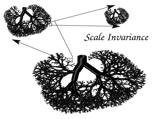
- ** All the methods are developed in a way to capture "invariances" within categories of interest**
- translation invariance
- rotation invariance
- scale invariance
- Deformation
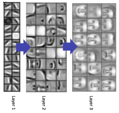
- Hierarchical Representation and Compositionality
- Text
- Video
- A Building
- Cities
In [2]:
N = 256
t = np.arange(N)
fi = .1*t
r = 1
z = np.cos(.1*t)
z1 = np.cos(.1*(t-30))
# .0*np.random.rand(N)
plt.plot(z)
plt.plot(z1)
Out[2]:
[<matplotlib.lines.Line2D at 0x11265ed10>]


Fourier Analysis is among the most fundamental methods in this field, developed in early 19th century
Interplay between Time and Frequency domains!
Essentially is says it is possible to represent any integrable function as a linear sum of sinosoidal functions with different frequencies
Much related with more general concepts such as Taylor Series: https://en.wikipedia.org/wiki/Taylor_series
Fourier Series as Harmonic Analysis
Examples of known functions


Source = https://gist.github.com/amroamroamro/617305c05001caffc8d0
A more interactive version


An important concept
Euler's formula
 It manages to encapsulate both cosine and sine function in a single complex exponentials.
https://en.wikipedia.org/wiki/Euler%27s_formula#Using_power_series
It manages to encapsulate both cosine and sine function in a single complex exponentials.
https://en.wikipedia.org/wiki/Euler%27s_formula#Using_power_series
In [3]:
#Complex Exponentials
N = 256
t = np.arange(N)
fi = .1*t
r = 1
cos = np.cos(.1*t)
sin = np.sin(.1*t)
ex = cos + 1j*sin
plt.plot(cos,linewidth=3)
plt.plot(np.real(ex),'.r')
plt.plot(np.imag(ex),'.g')
Out[3]:
[<matplotlib.lines.Line2D at 0x117b7aad0>]


In [4]:
#Base Filters 1D
def base_filter_1D(N):
    dd = -2*np.pi/N
    w = np.exp(dd*1j)
#     w = np.exp(-2*np.pi*1j/N)

    W = np.ones((N,N),dtype=complex)

    for i in range(N):
        for j in range(N):
            W[i,j] = np.power(w,i*j)

#     W = W/np.sqrt(N)
    return W


N = 4
W = base_filter_1D(N)
print np.around(W,decimals=3)
[[ 1.+0.j  1.+0.j  1.+0.j  1.+0.j]
 [ 1.+0.j  0.-1.j -1.-0.j -0.+1.j]
 [ 1.+0.j -1.-0.j  1.+0.j -1.-0.j]
 [ 1.+0.j -0.+1.j -1.-0.j  0.-1.j]]
In [5]:
def DFT_1D_basis_vis(i):
    fig = plt.figure(figsize=(10,5))
    plt.subplot(1,2,1)
    #Real Part of the vector
    plt.plot(np.real(W)[i],'r')
    #Imaginary Part of the vector
    plt.title('real part')
    plt.axis('off')
    plt.subplot(1,2,2)
    plt.title('imaginary part')
    plt.plot(np.imag(W)[i],'b')
    plt.axis('off')
N = 256
W = base_filter_1D(N)
interact(DFT_1D_basis_vis,i=(0,N-1,1));

In [6]:
fig = plt.figure(figsize=(10,10))
for i in range(16):
    plt.subplot(4,4,i+1)
    plt.plot(np.real(W)[i],'r')
    plt.plot(np.imag(W)[i],'b')
    plt.axis('off')

In [7]:
# They are orthogonal basis
#Each row of W is a basis

#Orthogonal Basis
a = np.imag(W)[2].dot(np.imag(W)[1])
print np.around(a)


#Sin and Cos
a = np.real(W)[2].dot(np.imag(W)[1])
print np.around(a)
-0.0
-0.0
Now from Time domain to Frequency domain
In [8]:
N = 128
t = np.arange(N)
x = 1*np.sin(.05*t) + 1*np.cos(5*t+.1)
plt.plot(x)
Out[8]:
[<matplotlib.lines.Line2D at 0x1189a0fd0>]

In [9]:
#DFT 1D
# Now we can transform this original signals to a new vector space based on fourier base patterns
# How to transform the original signal (DATA) to a new basis system
W = base_filter_1D(N)
X1 = W.dot(x)
# plt.plot(X,'.r')
plt.subplot(3,1,1)
plt.plot(x,'.-');
plt.title('time domain');
plt.subplot(3,1,2)
plt.plot(np.real(X1),'.');
plt.title('frequencey domain real part')
plt.subplot(3,1,3)
plt.plot(np.imag(X1),'.');
plt.title('frequencey domain imaginary part')
plt.tight_layout()

Fast Fourier Transform (FFT) in Numpy
In [10]:
plt.plot(np.abs(np.real(X1)),'or');


X = np.fft.fft(x)
plt.plot(np.abs(np.real(X)),'*b',markersize=3);

In [11]:
# Two signals have the same frequencies but with a shift in time
N = 256
t = np.arange(N)
x1 = .4*np.sin(1*t+.1) + .6*np.cos(-15*t+.1) + .3*np.random.rand(N)
x2 = .4*np.sin(1*(t-2)+.1) + .6*np.cos(-15*(t-16)+.1) + .1*np.random.rand(N)
plt.plot(x1)
plt.plot(x2)
Out[11]:
[<matplotlib.lines.Line2D at 0x119273cd0>]

In [12]:
W = base_filter_1D(N)
X1 = W.dot(x1)
X2 = W.dot(x2)
In [13]:
plt.plot(np.abs(np.absolute(X1)),'b');
plt.plot(np.abs(np.absolute(X2)),'g');

In [14]:
N = 128
t = np.arange(N)
x = 1*np.sin(5*t)

W = base_filter_1D(N)
X = W.dot(x)
W_inv = np.linalg.inv(W)

def reconstruct_signal(howmanybasis=1):
    x_r = W_inv[:,:howmanybasis].dot(X[:howmanybasis])
    plt.plot(x[:],'b');
    plt.plot(x_r[:],'r--');
    plt.ylim(-1,1)
interact(reconstruct_signal,howmanybasis=(0,N-1,1));

In [15]:
N = 128
t = np.arange(N)
x = 1*np.sin(.05*t) + 1*np.cos(.15*t+.1)  + .83*np.random.rand(N)

plt.plot(x[:],'b');

In [16]:
X  = np.fft.fft(x)
# plt.hist(X,bins=100);
plt.plot(np.absolute(X),'.');

In [17]:
def denoise(howmany=1):
    X  = np.fft.fft(x)
    X[np.argsort(-1*np.absolute(X))[howmany:]]=0
    plt.plot(np.fft.ifft(X),'r',linewidth=3)
    plt.plot(x)
interact(denoise,howmany=(0,N,1));

2D Fourier Transform
In [18]:
N = 32
W1D = base_filter_1D(N)
def base_filter2d_vis(u=1,v=1):

    r = W1D[u][np.newaxis,:].T
    c = W1D[v][np.newaxis,:]
    W2 = r.dot(c)
    fig = plt.figure(figsize=(15,7))
    plt.subplot(1,2,1)
    plt.title('Real Part(CoSine Wave)')
    plt.imshow(np.real(W2),cmap=plt.cm.gray)
    plt.axis('off')
    plt.subplot(1,2,2)
    plt.title('Imaginary Part (Sine Wave)')
    plt.axis('off')
    plt.imshow(np.imag(W2),cmap=plt.cm.gray)
In [19]:
interact(base_filter2d_vis,u=(0,N-1,1),v=(0,N-1,1));

In [20]:
#Base Filters 2D
def base_filter_2D(N):
    W1D = base_filter_1D(N)*np.sqrt(N)
    W2D = np.ones((N,N,N,N),dtype=complex)

    for u in range(0,N):
        for v in range(0,N):
            r = W1D[u][np.newaxis,:].T
            c = W1D[v][np.newaxis,:]
            W2D[u,v,:,:] = r.dot(c)
    W2D = W2D/(np.sqrt(N*N))
    return W2D
Base Filters Dictionary
- Note that these base filters are defined independent of the data!
In [21]:
N = 8
W2D = base_filter_2D(N)
print W2D.shape
fig = plt.figure(figsize=(7,7))
k =1
for u in range(0,N):
    for v in range(0,N):
        W2 = W2D[u,v,:,:]
        plt.subplot(N,N,k)
        plt.imshow(np.real(W2),cmap=plt.cm.gray)
#         plt.imshow(np.imag(W2),cmap=plt.cm.gray)
        k = k +1
        plt.axis('off')
(8, 8, 8, 8)

In [22]:
#DFT  in 2D is much more time consuming.
# Each cell is calculate as the sum of the dot product of base filter corresponding of that cell and the whole image
## Very slow: Don't use it :)
def DFT2D(W2D,img):
    N = img.shape[0]
    M = img.shape[1]
    img_fr = np.ones((N,N),dtype=complex)
    for i in range(N):
        for j in range(M):
            img_fr[i,j]= W2D[i,j,:,:].dot(img).sum()
    return img_fr

def InverseDFT2D(howmanybasis=1):
    img_rec = img
    for u in range(howmanybasis):
        for v in range(howmanybasis):
            W = W2D[u,v,:]
            W_inv = np.linalg.inv(W)
            for i in range(N):
                for j in range(M):
                    img_rec[i,j]= W_inv.dot(IMG[:howmanybasis,:howmanybasis]).sum()
In [35]:
from skimage import data
from skimage.color import rgb2gray

fig = plt.figure(figsize=(9,6))

img = data.astronaut()
img = rgb2gray(img)
img = img
# + np.random.rand(img.shape[0],img.shape[1])


N = img.shape[0]
img = np.zeros((N, N))

x = 60
y = 60


for i in range(20):
    indx = np.random.randint(x,N-x)
    indy = np.random.randint(y,N-y)
    img[indx:indx+x,indy:indy+y] = 1


plt.subplot(2,3,1)

plt.imshow(img,cmap=plt.cm.gray);
plt.axis('off')

F_img = np.fft.fft2(img)
F_img = np.fft.fftshift(F_img)
plt.subplot(2,3,4);
plt.imshow(np.log(np.absolute(F_img)));
plt.axis('off');

Nx = img.shape[0]
Ny = img.shape[1]

x  =30
y = 30
High_pass_freq =  F_img.copy()
High_pass_freq[Nx/2-x:Nx/2+x,Ny/2-y:Ny/2+y] = 0

High_pass_img = np.fft.ifft2(High_pass_freq)
plt.subplot(2,3,2);
plt.title('High Pass Filter');
plt.imshow(np.absolute(High_pass_img),cmap=plt.cm.gray);
plt.axis('off');


plt.subplot(2,3,5);
plt.imshow(np.log(np.absolute(High_pass_freq)));
plt.axis('off');


Low_pass_freq =  F_img.copy()
Low_pass_freq[Nx/2+x:,:] = 0
Low_pass_freq[:,:Ny/2-y] = 0
Low_pass_freq[:Nx/2-x,:] = 0
Low_pass_freq[:,Ny/2+y:] = 0

Low_pass_img = np.fft.ifft2(Low_pass_freq)
plt.subplot(2,3,3);
plt.title('Low Pass Filter');
plt.imshow(np.absolute(Low_pass_img),cmap=plt.cm.gray);
plt.axis('off');


plt.subplot(2,3,6);

plt.imshow(np.log(np.absolute(Low_pass_freq)));
plt.axis('off');

Effect of Shift
In [78]:
# Example 1
N = 128
x = 5
y = 10
img = np.zeros((128,128))
img[N/2-x:N/2+x,N/2-y:N/2+y] = 1
plt.subplot(1,2,1);
plt.imshow(img,cmap=plt.cm.gray);
plt.axis('off');


plt.subplot(1,2,2);
F_img = np.fft.fft2(img)
#To shift low pass (lower freq) to the center
F_img = np.fft.fftshift(F_img)
plt.imshow(np.log(np.absolute(F_img)));
plt.axis('off');

In [79]:
# Example 1
# With shift stil the patters are similar in freq domain
N = 128
x = 5
y = 10
img = np.zeros((128,128))
img[N/5-x:N/5+x,N/2-y:N/2+y] = 1
plt.subplot(1,2,1);
plt.imshow(img,cmap=plt.cm.gray);


plt.subplot(1,2,2);
F_img = np.fft.fft2(img)

#To shift low pass (lower freq) to the center
F_img = np.fft.fftshift(F_img);
plt.imshow(np.log(np.absolute(F_img)));

In [80]:
# Example 1
# With shift stil the patters are similar in freq domain
N = 128
x = 5
y = 5
img = np.zeros((128,128))

for i in range(20):
    indx = np.random.randint(x,N-x)
    indy = np.random.randint(y,N-y)
    img[indx:indx+x,indy:indy+y] = 1
plt.subplot(2,2,1);
plt.imshow(img,cmap=plt.cm.gray);
plt.axis('off');

plt.subplot(2,2,2);
F_img = np.fft.fft2(img)

#To shift low pass (lower freq) to the center
F_img = np.fft.fftshift(F_img)
plt.imshow(np.log(np.absolute(F_img)));
plt.axis('off');


img = np.zeros((128,128))

for i in range(20):
    indx = np.random.randint(x,N-x)
    indy = np.random.randint(y,N-y)
    img[indx:indx+x,indy:indy+y] = 1
plt.subplot(2,2,3);
plt.imshow(img,cmap=plt.cm.gray);
plt.axis('off');


plt.subplot(2,2,4);
F_img = np.fft.fft2(img)

#To shift low pass (lower freq) to the center
F_img = np.fft.fftshift(F_img)
plt.imshow(np.log(np.absolute(F_img)));
plt.axis('off');

So in principle we can use the representations at the frequency domain as the variables for our other ML tasks such as classification.
However, it doesn't work well for Scale variations
In [84]:
# Example 1
# With shift stil the patters are similar in freq domain
N = 128
x = 5
y = 5
img = np.zeros((128,128))

for i in range(2):
    indx = np.random.randint(x,N-x)
    indy = np.random.randint(y,N-y)
    img[indx:indx+x,indy:indy+y] = 1


# img = np.zeros((128,128))
# img[N/2-x:N/2+x,N/2-y:N/2+y] = 1

plt.subplot(2,2,1);
plt.imshow(img,cmap=plt.cm.gray);
plt.axis('off');

plt.subplot(2,2,2);
F_img = np.fft.fft2(img)

#To shift low pass (lower freq) to the center
F_img = np.fft.fftshift(F_img)
plt.imshow(np.log(np.absolute(F_img)));
plt.axis('off');


img = np.zeros((128,128))
x = 15
y = 15

# img = np.zeros((128,128))
# img[N/2-x:N/2+x,N/2-y:N/2+y] = 1

for i in range(2):
    indx = np.random.randint(x,N-x)
    indy = np.random.randint(y,N-y)
    img[indx:indx+x,indy:indy+y] = 1
plt.subplot(2,2,3);
plt.imshow(img,cmap=plt.cm.gray);
plt.axis('off');


plt.subplot(2,2,4);
F_img = np.fft.fft2(img)

#To shift low pass (lower freq) to the center
F_img = np.fft.fftshift(F_img)
plt.imshow(np.log(np.absolute(F_img)));
plt.axis('off');

TO improve any of these exceptions there have been many different methods developed and this field sometimes is called "Feature Engineering"
For Example
- Wavelets
- Scattering Wavelets
- SIFT https://en.wikipedia.org/wiki/Scale-invariant_feature_transform
- Many others
But there is a conceptual limit in these approaches.
As we can see filters in Fourier are just marginally effected by the data (via its dimension)
Conceptually, Fouries Transform is at the same level as Polynomial regression, where there is a parametric structure imposed to data set.
PCA as a limited data driven feature learning doesn't work.
In [85]:
N = 30
x = 2
y = 2
nsq = 30
dim = N*N
image_shape = [N,N]
pattern_image = np.zeros((10000,dim))
for k in range(pattern_image.shape[0]):
    img = np.zeros((N,N))
    for i in range(20):
        indx = np.random.randint(x,N-x)
        indy = np.random.randint(y,N-y)
        img[indx:indx+x,indy:indy+y] = 1
    pattern_image[k,:]= img.flatten()
In [86]:
from sklearn.decomposition import PCA
X = pattern_image
pca = PCA()
pca.fit(X)
Out[86]:
PCA(copy=True, iterated_power='auto', n_components=None, random_state=None,
  svd_solver='auto', tol=0.0, whiten=False)
In [87]:
fig = plt.figure(figsize=(7,7))
W_pca = pca.components_
for i in range(100):
    plt.subplot(10,10,i+1)
    plt.imshow((W_pca[i]).reshape(image_shape),cmap=plt.cm.gray);
    plt.axis('off')
    plt.yticks([]);

In [52]:
N = 8
W2D = base_filter_2D(N)
print W2D.shape
fig = plt.figure(figsize=(7,7))
k =1
for u in range(0,N):
    for v in range(0,N):
        W2 = W2D[u,v,:,:]
        plt.subplot(N,N,k)
        plt.imshow(np.real(W2),cmap=plt.cm.gray)
#         plt.imshow(np.imag(W2),cmap=plt.cm.gray)
        k = k +1
        plt.axis('off')
(8, 8, 8, 8)

Convolutional Neural Networks (CNN) are seemingly a very good answer