Data Driven Modeling
### PhD seminar series at Chair for Computer Aided Architectural Design (CAAD), ETH Zurich
Topics to be discussed
- Data Clustering
- K-Means
- Limits and Extensions
- Probabilistinc Clustering
- Density based clustering
- Fundamental limits to classical notion of clusters and community detection
- Clustering as feature learning in comparison to PCA and sparse coding
- Clustering as space indexing
- Vector Quantization
- Introduction to Self Organizing Maps
In [106]:
import warnings
warnings.filterwarnings("ignore")
import pandas as pd
import numpy as np
from matplotlib import pyplot as plt
pd.__version__
import sys
from scipy import stats
%matplotlib inline
Data Clustering Problem
In [107]:
# A two dimensional example
fig = plt.figure()

N = 50
d0 = 1.6*np.random.randn(N,2)
d0[:,0]= d0[:,0] - 3
plt.plot(d0[:,0],d0[:,1],'.b')

d1 = 1.6*np.random.randn(N,2)+7.6
plt.plot(d1[:,0],d1[:,1],'.b')

d2 = 1.6*np.random.randn(N,2)
d2[:,0]= d2[:,0] + 5
d2[:,1]= d2[:,1] + 1
plt.plot(d2[:,0],d2[:,1],'.b')

d3 = 1.6*np.random.randn(N,2)
d3[:,0]= d3[:,0] - 5
d3[:,1]= d3[:,1] + 4
plt.plot(d3[:,0],d3[:,1],'.b')


d4 = 1.8*np.random.randn(N,2)
d4[:,0]= d4[:,0] - 15
d4[:,1]= d4[:,1] + 14
plt.plot(d4[:,0],d4[:,1],'.b')


d5 = 1.8*np.random.randn(N,2)
d5[:,0]= d5[:,0] + 25
d5[:,1]= d5[:,1] + 14
plt.plot(d5[:,0],d5[:,1],'.b')
Data1 = np.concatenate((d0,d1,d2,d3,d4,d5))
fig.set_size_inches(7,7)

In [4]:
# A two dimensional example
fig = plt.figure()
plt.plot(d0[:,0],d0[:,1],'.')
plt.plot(d1[:,0],d1[:,1],'.')
plt.plot(d2[:,0],d2[:,1],'.')
plt.plot(d3[:,0],d3[:,1],'.')
plt.plot(d4[:,0],d4[:,1],'.')
plt.plot(d5[:,0],d5[:,1],'.')


mu0= d0.mean(axis=0)[np.newaxis,:]
mu1= d1.mean(axis=0)[np.newaxis,:]
mu2= d2.mean(axis=0)[np.newaxis,:]
mu3= d3.mean(axis=0)[np.newaxis,:]
mu4= d4.mean(axis=0)[np.newaxis,:]
mu5= d5.mean(axis=0)[np.newaxis,:]
mus = np.concatenate((mu0,mu1,mu2,mu3,mu4,mu5),axis=0)

plt.plot(mus[:,0],mus[:,1],'o',markersize=10)

fig.set_size_inches(7,7)

In [108]:
N = 50
x1= np.random.normal(loc=0,scale=1,size=N)[:,np.newaxis]
x2= np.random.normal(loc=0,scale=5,size=N)[:,np.newaxis]
y = 3*x1 + np.random.normal(loc=.0, scale=.7, size=N)[:,np.newaxis]
# y = 2*x1
# y = x1*x1 + np.random.normal(loc=.0, scale=0.6, size=N)[:,np.newaxis]
# y = 2*x1*x1

fig = plt.figure(figsize=(7,7))
ax1= plt.subplot(111)
plt.plot(x1,y,'or',markersize=10,alpha=.4 );

In [109]:
def linear_regressor(a,b):
    # y_ = ax+b
    mn = np.min(x1)
    mx = np.max(x1)
    xrng =  np.linspace(mn,mx,num=500)
    y_ = [a*x + b for x in xrng]


    fig = plt.figure(figsize=(7,7))
    ax1= plt.subplot(111)
    plt.plot(x1,y,'or',markersize=10,alpha=.4 );
    plt.xlabel('x1');
    plt.ylabel('y');
    plt.plot(xrng,y_,'-b',linewidth=1)
#     plt.xlim(mn-1,mx+1)
#     plt.ylim(np.min(y)+1,np.max(y)-1)

    yy = [a*x + b for x in x1]

    [plt.plot([x1[i],x1[i]],[yy[i],y[i]],'-r',linewidth=1) for i in range(len(x1))];
#     print 'average squared error is {}'.format(np.mean((yy-y)**2))
In [110]:
from ipywidgets import interact, HTML, FloatSlider
interact(linear_regressor,a=(-3,6,.2),b=(-2,5,.2));


In [111]:
import scipy.spatial.distance as DIST
def Assign_Sets(mus,X):
    Dists = DIST.cdist(X,mus)
    ind_sets = np.argmin(Dists,axis=1)
    min_dists = np.min(Dists,axis=1)
    energy = np.sum(min_dists**2)
    return ind_sets, energy


def update_mus(ind_sets,X,K):

    n_mus = np.zeros((K,X.shape[1]))
    for k in range(K):
        ind = ind_sets==k
        DD = X[ind]
        if DD.shape[0]>0:
            n_mus[k,:]=np.mean(DD,axis=0)
        else:
            continue


    return n_mus

def Visualize_assigned_sets(mu00=None,mu01=None,mu10=None,mu11=None,mu20=None,mu21=None):
    mus0 = np.asarray([mu00,mu10,mu20])[:,np.newaxis]
    mus1 = np.asarray([mu01,mu11,mu21])[:,np.newaxis]
    mus = np.concatenate((mus0,mus1),axis=1)
    ind_sets,energy = Assign_Sets(mus,X)

    fig = plt.figure(figsize=(7,7))
    ax1= plt.subplot(111)

    for k,mu in enumerate(mus):
        ind = ind_sets==k
        DD = X[ind]
        plt.plot(DD[:,0],DD[:,1],'.',markersize=10,alpha=.4 );
        plt.plot(mu[0],mu[1],'ob',markersize=10,alpha=.4 );

        [plt.plot([DD[i,0],mu[0]],[DD[i,1],mu[1]],'-k',linewidth=.1) for i in range(len(DD))];
In [112]:
X = Data1.copy()
mn = np.min(X,axis=0)
mx = np.max(X,axis=0)
R = mx-mn

# Assume K = 3

from ipywidgets import interact, HTML, FloatSlider
interact(Visualize_assigned_sets,mu00=(mn[0],mx[0],1),mu01=(mn[1],mx[1],1),
                        mu10=(mn[0],mx[0],1),mu11=(mn[1],mx[1],1),
                        mu20=(mn[0],mx[0],1),mu21=(mn[1],mx[1],1));

Although it looks simple, this is a hard problem and there is no exact solution for it.
In order to solve this we need to use heuristic methods. For example the following steps:
* initiate K random centers and assign each data point to its closest center.
* Now we have K sets. Within each sets, update the location of the center to minimize the above objective function.
* Due to the structure of these objective function, the mean vector of each set gives the minimum value.
* Therefore, simply update the locations of center points to the mean vector of each set.
* repeat the above steps, until the difference between two sequential centers are less than a threshhold
In [113]:
K =5
mus_t = np.zeros((K,X.shape[1]))
mus_0 = np.zeros((K,X.shape[1]))
fig = plt.figure(figsize=(16,7));
thresh = .01
mus_0[:,0] = mn[0] + np.random.random(size=K)*R[0]
mus_0[:,1] = mn[1] + np.random.random(size=K)*R[1]
mus_t = mus_0.copy()
diff = 1000
plt.subplot(1,2,1);
plt.plot(X[:,0],X[:,1],'.');
[plt.plot(mus_t[i,0],mus_t[i,1],'or',markersize=15,linewidth=.1,label='initial') for i in range(K)];
all_diffs =  []
all_energies = []
while diff> thresh:
    ind_sets, energy = Assign_Sets(mus_t,X)
    all_energies.append(energy)
    mus_tp = update_mus(ind_sets,X,K)
    diff = np.abs(mus_t- mus_tp).sum(axis=1).sum().copy()
    [plt.plot([mus_t[i,0],mus_tp[i,0]],[mus_t[i,1],mus_tp[i,1]],'-og',markersize=5,linewidth=.8) for i in range(K)];

    all_diffs.append(diff)
#         print diff
    mus_t= mus_tp.copy()
[plt.plot(mus_tp[i,0],mus_tp[i,1],'ob',markersize=15,linewidth=.1,label='final') for i in range(K)];

# # plt.legend(bbox_to_anchor=(1.1,1.));
# plt.xlabel('x');
# plt.ylabel('y');
# plt.subplot(3,1,2);
# plt.plot(all_diffs);
# plt.ylabel('average abs difference between two results');
# plt.xlabel('iterations');


plt.subplot(1,2,2);
plt.plot(all_energies,'-.r');
plt.ylabel('energy level');
plt.xlabel('iterations');
Out[113]:
<matplotlib.text.Text at 0x11c7c14d0>

In [114]:
def K_means(X,K):
    mus_t = np.zeros((K,X.shape[1]))
    mus_0 = np.zeros((K,X.shape[1]))
    thresh = .01
    mus_0[:,0] = mn[0] + np.random.random(size=K)*R[0]
    mus_0[:,1] = mn[1] + np.random.random(size=K)*R[1]
    mus_t = mus_0.copy()
    diff = 1000
    all_diffs =  []
    all_energies = []
    while diff> thresh:
        ind_sets, energy = Assign_Sets(mus_t,X)
        all_energies.append(energy)
        mus_tp = update_mus(ind_sets,X,K)
        diff = np.abs(mus_t- mus_tp).sum(axis=1).sum().copy()

        all_diffs.append(diff)

        mus_t= mus_tp.copy()
    return mus_t,all_diffs,all_energies
The effect of the chosen K
In [115]:
K =5

def visualize_Kmeans(K=5):
    centers, diffs, energies = K_means(X,K)
    ind_sets,energy = Assign_Sets(centers,X)
    fig = plt.figure()
    for k in range(K):
#         print
        ind = ind_sets==k
        DD = X[ind]
        plt.plot(DD[:,0],DD[:,1],'o',alpha=0.5, markersize=4,color=plt.cm.RdYlBu_r(float(k)/K));
        plt.plot(centers[k,0],centers[k,1],marker='o',markersize=15,alpha=1.,color=plt.cm.RdYlBu_r(float(k)/K));
    fig.set_size_inches(7,7)
In [116]:
from ipywidgets import interact, HTML, FloatSlider
X = Data1
interact(visualize_Kmeans,K=(1,10,1));

Assumptions and Extensions to K-Means
- How to select K in advance (metaparameter issue)
- e.g. Elbow method
- Similarity measures
- Shape of the clusters
- fuzzy k-means
- Hierarchical Clustering
- ** Pribabilistic Clustering a.k.a Mixture Models**
- Sensitivity to outliers
- Density based algorithms such as DBSCAN
Probabilistic Clustering
With different densities and shapes
Gaussian Mixture Models
- Gaussian Mixture Model: To learn the distribution of the data as a weighted sum of several globally defined Gaussian Distributions:
$$g(X) = \sum_{i = 1}^k p_i. g(X,\theta_i)$$
$ g(X,\theta_i)$ is a parametric known distribution (e.g. Gaussian) and $p_i$ is the share of each of them.
In [117]:
import sklearn.mixture.gmm as GaussianMixture
gmm = GaussianMixture.GMM(n_components=K, random_state=0,covariance_type='full')
In [118]:
def GMM_cluster(K=5):
    from matplotlib.colors import LogNorm
    import sklearn.mixture.gmm as GaussianMixture
    gmm = GaussianMixture.GMM(n_components=K, random_state=0,covariance_type='full')
    gmm.fit(X)
    Clusters = gmm.predict(X)
    fig = plt.figure()
    for k in range(K):
        ind = Clusters==k
        DD = X[ind]
        plt.plot(DD[:,0],DD[:,1],'o',alpha=1., markersize=4,color=plt.cm.RdYlBu_r(float(k)/K));
        plt.plot(gmm.means_[k,0],gmm.means_[k,1],marker='o',markersize=10,alpha=1.,color=plt.cm.RdYlBu_r(float(k)/K));
#     plt.plot(centers[:,0],centers[:,1],'or',alpha=1., markersize=15);
    fig.set_size_inches(7,7)


    x = np.linspace(X[:,0].min()-2,X[:,0].max()+2,num=200)
    y = np.linspace(X[:,1].min()-2,X[:,1].max()+2,num=200)
    X_, Y_ = np.meshgrid(x, y)
    XX = np.array([X_.ravel(), Y_.ravel()]).T
    Z = gmm.score_samples(XX)
    Z = -1*Z[0].reshape(X_.shape)

    # plt.imshow(Z[::-1], cmap=plt.cm.gist_earth_r,)
    # plt.contour(Z[::-1])
    CS = plt.contour(X_, Y_, Z, norm=LogNorm(vmin=1.0, vmax=1000.0),
                     levels=np.logspace(0, 3, 10),cmap=plt.cm.RdYlBu_r);
In [119]:
from ipywidgets import interact, HTML, FloatSlider
X = Data1
pttoptdist = DIST.cdist(X,X)
interact(GMM_cluster,K=(1,6,1));

In [120]:
def DBSCAN_1(eps=.5, MinPts=10):
    Clusters = np.zeros((X.shape[0],1))
    C = 1
    processed = np.zeros((X.shape[0],1))
    for i in range(X.shape[0]):
        if processed[i]==0:
            inds_neigh = pttoptdist[i]<=eps
            pointers = inds_neigh*range(X.shape[0])
            pointers = np.unique(pointers)[1:]

            if pointers.shape[0]>= MinPts:
                processed[i]==1
                Clusters[i]=C
                #it is a core point and not processed/clustered yet
                # A new cluster
                #Find other members of this cluster
                counter = 0
                while (counter < pointers.shape[0]):
                    ind = pointers[counter]
#                     print i,pointers.shape
                    if processed[ind]==0:
                        processed[ind] = 1
                        inds_neigh_C = pttoptdist[ind]<= eps
                        pointers_ = inds_neigh_C*range(X.shape[0])
                        pointers_ = np.unique(pointers_)[1:]
                        if pointers_.shape[0]>= MinPts:
                            pointers = np.concatenate((pointers,pointers_))
                    if Clusters[ind] == 0:
                        Clusters[ind] = C
                    counter = counter +1

                C = C + 1

            else:
                # for now it is noise, but it might be connected later as non-core point
                Clusters[i]=0

        else:
            continue


    fig = plt.figure(figsize=(7,7))
    ax1= plt.subplot(111)
    K =np.unique(Clusters).shape[0]-1
    for i,k in enumerate(np.unique(Clusters)[:]):
        ind = Clusters==k
        DD = X[ind[:,0]]

        #cluster noise
        if k==0:
            plt.plot(DD[:,0],DD[:,1],'.k',markersize=5,alpha=1 );
        else:
            plt.plot(DD[:,0],DD[:,1],'o',markersize=10,alpha=.4,color=plt.cm.RdYlBu_r(float(i)/K) );


#     return Clusters
In [121]:
from ipywidgets import interact, HTML, FloatSlider
X = Data1
pttoptdist = DIST.cdist(X,X)
interact(DBSCAN_1,eps=(.05,3,.1),MinPts=(4,20,1));

In [122]:
dlen = 700
tetha = np.random.uniform(low=0,high=2*np.pi,size=dlen)[:,np.newaxis]
X1 = 3*np.cos(tetha)+ .22*np.random.rand(dlen,1)
Y1 = 3*np.sin(tetha)+ .22*np.random.rand(dlen,1)
D1 = np.concatenate((X1,Y1),axis=1)

X2 = 1*np.cos(tetha)+ .22*np.random.rand(dlen,1)
Y2 = 1*np.sin(tetha)+ .22*np.random.rand(dlen,1)
D2 = np.concatenate((X2,Y2),axis=1)

X3 = 5*np.cos(tetha)+ .22*np.random.rand(dlen,1)
Y3 = 5*np.sin(tetha)+ .22*np.random.rand(dlen,1)
D3 = np.concatenate((X3,Y3),axis=1)

X4 = 8*np.cos(tetha)+ .22*np.random.rand(dlen,1)
Y4 = 8*np.sin(tetha)+ .22*np.random.rand(dlen,1)
D4 = np.concatenate((X4,Y4),axis=1)


Data3 = np.concatenate((D1,D2,D3,D4),axis=0)

fig = plt.figure()
plt.plot(Data3[:,0],Data3[:,1],'ob',alpha=0.2, markersize=4)
fig.set_size_inches(7,7)

In [123]:
from ipywidgets import interact, HTML, FloatSlider
X = Data3
interact(visualize_Kmeans,K=(1,10,1));

In [125]:
from ipywidgets import interact, HTML, FloatSlider
X = Data3
pttoptdist = DIST.cdist(X,X)
interact(DBSCAN_1,eps=(.1,2,.1),MinPts=(4,20,1));

However, since DBSCAN has it own limit: It assumes a global ratio for density
In [126]:
# A two dimensional example
fig = plt.figure()

N = 280
d0 = .5*np.random.randn(N,2) + [[3,2]]
d0 = .5*np.random.multivariate_normal([3,2],[[.8,.6],[.71,.7]],N)
plt.plot(d0[:,0],d0[:,1],'.b')


d1 = .6*np.random.randn(1*N,2)
plt.plot(d1[:,0],d1[:,1],'.b')

d2 = .5*np.random.randn(2*N,2)+[[-3,2]]

plt.plot(d2[:,0],d2[:,1],'.b')

# d3 = 1.6*np.random.randn(N,2)
# d3[:,0]= d3[:,0] - 5
# d3[:,1]= d3[:,1] + 4
# plt.plot(d3[:,0],d3[:,1],'.b')


Data2 = np.concatenate((d0,d1,d2))
fig.set_size_inches(7,7)

In [128]:
from ipywidgets import interact, HTML, FloatSlider
X = Data2
pttoptdist = DIST.cdist(X,X)
interact(DBSCAN_1,eps=(.05,3,.05),MinPts=(4,20,1));

In [129]:
from ipywidgets import interact, HTML, FloatSlider
X = Data2
interact(visualize_Kmeans,K=(1,3,1));

More than that, topological algorithms like DBSCAN have fundamental limits:
They are usually developed based on synthetic data sets, which usually never happens in reality
Further, they believe in some kind of underlying true groups!!! Or some kind of Idealized set up such as having perfect communities!!!
More Important: They have NO data Abstraction and NO Generalization
Attention to these issues can be a turining point in the notion of clustering
If we look at K-means ojective function
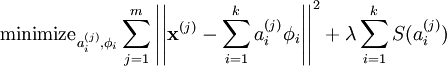
In comparison to Sparse Coding (SC) objective function
Or to PCA
$$ x = yP $$
Or to GMM
$$g(X) = \sum_{i = 1}^k p_i. g(X,\theta_i)$$
We can think of cluster centers as new "fictional" dimensions.
Then, similar to PCA or SC, the identified cluster centers can be used as dimensionality of the data points.
Previous floor plan example that we had with PCA and SC
In [76]:
from sklearn.datasets import fetch_mldata


from sklearn.datasets import fetch_olivetti_faces


#Chairs
path = "./Data/chairs.csv"
D = pd.read_csv(path,header=None)
image_shape = (64,64)
Images = D.values[:]
print Images.shape


# floorplan
path = "./Data/1000FloorPlans.csv"
D = pd.read_csv(path,header=None)
image_shape = (50, 50)
faces = D.values[:]
# faces[faces>0] = -1
# faces[faces==0] = 1
# faces[faces==-1] = 0
Images = faces[:]
print Images.shape


# # Mnist data set
# image_shape = (28, 28)
# dataset = fetch_mldata('MNIST original')
# # faces = dataset.data
# X = faces[:]
# X.shape


fig = plt.figure(figsize=(12,12))
for i in range(25):
    plt.subplot(5,5,i+1)
    plt.imshow(Images[i].reshape(image_shape),cmap=plt.cm.gray);
    plt.xticks([]);
    plt.yticks([]);
plt.tight_layout()
(696, 4096)
(999, 2500)

In [77]:
from sklearn.feature_extraction.image import extract_patches_2d
rng = np.random.RandomState(0)
patch_size = (16, 16)
buffer = []
for img in Images:
        data = extract_patches_2d(img.reshape(image_shape), patch_size, max_patches=50,
                                  random_state=rng)
        data = np.reshape(data, (len(data), -1))
        buffer.extend(data)
Patch_Images = np.asarray(buffer)
print Patch_Images.shape
(49950, 256)
In [78]:
fig = plt.figure(figsize=(12,12))
for i in range(25):
    plt.subplot(5,5,i+1)
    plt.imshow(Patch_Images[1000+i].reshape(patch_size),cmap=plt.cm.gray);
    plt.xticks([]);
    plt.yticks([]);
plt.tight_layout()

In [79]:
means = Patch_Images.mean(axis=1)[:,np.newaxis]
Vars = Patch_Images.std(axis=1)**2 +.05
denom = np.sqrt(Vars)[:,np.newaxis]
Patch_Images = (Patch_Images-means)/denom
# /
In [84]:
from sklearn.cluster import KMeans
kmeans = KMeans(n_clusters=200, random_state=0).fit(Patch_Images)
In [85]:
fig = plt.figure(figsize=(10,20))
for i in range(200):
    plt.subplot(20,10,i+1)
    plt.imshow(kmeans.cluster_centers_[i,:].reshape(patch_size),cmap=plt.cm.gray);
    plt.xticks([]);
    plt.yticks([]);
plt.tight_layout(h_pad=.01, w_pad=.01)

Another view to the problem of clustering
Are outliers bad things or good things?
Examples:
research communities and those research topics that don't belong to any group?
** Can we say outliers might be those who are ahead of their fields?
** What if we set our criteria based on the above clustering definition?**
** One tricky recent application of ML in peer review process: Quick pre-assessments of papers for their potential popularity!!!***
What if we say each obsevation is a potential communiy itself?
What if we increase K in K-means drastically
In [130]:
from ipywidgets import interact, HTML, FloatSlider
X = Data3
interact(visualize_Kmeans,K=(3,300,1));

In [131]:
from ipywidgets import interact, HTML, FloatSlider
X = Data1
interact(visualize_Kmeans,K=(200,300,1));

In order to do so, we invert the whole game of data clustering
we create an aribitrary ordered set of indexes and try to fit them to data, while having a "topology preserving" indexing.
This means, if two indices have similar label, they should index a similar area of data space and vice versa.
This is the original idea of Self Organizing Maps (SOM)
In [137]:
import sompylib.sompy as SOM
msz11 =15
msz10 = 10
X = Data1
som1 = SOM.SOM('', X, mapsize = [msz10, msz11],norm_method = 'var',initmethod='random')
som1.init_map()
som1.train(n_job = 1, shared_memory = 'no',verbose='final')
codebook1 = som1.codebook[:]
codebook1_n = SOM.denormalize_by(som1.data_raw, codebook1, n_method = 'var')
Total time elapsed: 0.080000 secodns
final quantization error: 0.071330
In [138]:
fig = plt.figure()
plt.plot(X[:,0],X[:,1],'ok',alpha=0.5, markersize=4);
K = som1.nnodes
for k in range(som1.nnodes):
    plt.plot(codebook1_n[k,0],codebook1_n[k,1],marker='o',markersize=10,alpha=1.,color=plt.cm.RdYlBu_r(float(k)/K));
fig.set_size_inches(7,7)

In [139]:
som1.hit_map()

In [140]:
som1.view_map(text_size=6,COL_SiZe=4)

This mechanism of indexing the space is called manifold learning and as we will see later SOM has lots of amazing capacities for many hig-dimensioanl data sets.
An example with high dimensional data
In [141]:
path = "./Data/rentalprice.csv"
D = pd.read_csv(path)
# D  = D[['Rent','ZIP','Year built','Living space','lng','lat']]
D.head()
Out[141]:
| Rent | ZIP | Type_Apartment | Type_Duplex | Type_Single house | Type_Studio | Rooms | Year built | Living space | lng | lat | |
|---|---|---|---|---|---|---|---|---|---|---|---|
| 0 | 645.0 | 5000 | 1.0 | 0.0 | 0.0 | 0.0 | 1.0 | 1954.0 | 28.0 | 8.041672 | 47.397999 |
| 1 | 1340.0 | 5000 | 1.0 | 0.0 | 0.0 | 0.0 | 4.0 | 1971.0 | 88.0 | 8.057444 | 47.379288 |
| 2 | 1380.0 | 5000 | 1.0 | 0.0 | 0.0 | 0.0 | 3.0 | 1968.0 | 69.0 | 8.057165 | 47.378022 |
| 3 | 1480.0 | 5000 | 1.0 | 0.0 | 0.0 | 0.0 | 3.5 | 1976.0 | 81.0 | 8.057974 | 47.400780 |
| 4 | 1500.0 | 5000 | 1.0 | 0.0 | 0.0 | 0.0 | 4.0 | 1968.0 | 80.0 | 8.057165 | 47.378022 |
In [ ]:
In [142]:
import sompylib.sompy as SOM
msz11 =40
msz10 = 40

X = D.values[:]

som1 = SOM.SOM('', X, mapsize = [msz10, msz11],norm_method = 'var',initmethod='pca')
som1.init_map()
som1.train(n_job = 1, shared_memory = 'no',verbose='final')
codebook1 = som1.codebook[:]
codebook1_n = SOM.denormalize_by(som1.data_raw, codebook1, n_method = 'var')
som1.compname= [D.columns]
Total time elapsed: 2.530000 secodns
final quantization error: 0.537370
In [143]:
som1.hit_map()

In [ ]:
In [144]:
som1.view_map(text_size=6,COL_SiZe=4)

How this inverts the notion of clustering and detection of communities and their outliers to the communities around individuals!
In [145]:
N = 50
x1= np.random.normal(loc=17,scale=5,size=N)[:,np.newaxis]
x2= np.random.normal(loc=0,scale=10,size=N)[:,np.newaxis]
y = 3*x1 + np.random.normal(loc=.0, scale=.4, size=N)[:,np.newaxis]

# x1 = np.random.uniform(size=N)[:,np.newaxis]
# y = np.sin(2*np.pi*x1**3)**3 + .1*np.random.randn(*x1.shape)

y =-.1*x1**3 + 2*x1*x1 + 2*np.sqrt(x1)+ 10*np.random.normal(loc=30.0, scale=4.7, size=len(x1))[:,np.newaxis]


degree= 2
from sklearn.preprocessing import PolynomialFeatures
from sklearn import linear_model
X_tr = x1[:].astype(float)
y_tr = y[:].astype(float)
poly = PolynomialFeatures(degree=degree)
X_tr_ = poly.fit_transform(X_tr)
regr = linear_model.LinearRegression()
regr.fit(X_tr_, y_tr)
X_pred = np.linspace(X_tr.min(),X_tr.max(),num=500)[:,np.newaxis]
X_pred_ = poly.fit_transform(X_pred)
y_pred = regr.predict(X_pred_)[:]
In [146]:
import sompylib.sompy as SOM
msz11 =20
msz10 = 20
X = np.concatenate((x1,y),axis=1)
som1 = SOM.SOM('', X, mapsize = [msz10, msz11],norm_method = 'var',initmethod='pca')
som1.init_map()
som1.train(n_job = 1, shared_memory = 'no',verbose='final')
codebook1 = som1.codebook[:]
codebook1_n = SOM.denormalize_by(som1.data_raw, codebook1, n_method = 'var')
Total time elapsed: 1.595000 secodns
final quantization error: 0.007808
In [147]:
fig = plt.figure()
fig.set_size_inches(14,7)
plt.subplot(1,2,1)
plt.title('data points vote for the line')
plt.plot(X_tr,y_tr,'.r',markersize=20,alpha=.4 );
plt.plot(X_pred,y_pred,'ok',markersize=3,alpha=.4 );


plt.subplot(1,2,2)
plt.title('each data point creates its own community')
plt.plot(X[:,0],X[:,1],'.r',alpha=0.5, markersize=20);
plt.plot(codebook1_n[:,0],codebook1_n[:,1],'ok',markersize=3,alpha=1.);
plt.tight_layout()
font = {'size'   : 12}
plt.rc('font', **font)
