PyCM Document
Version : 2.1
Table of contents
- Overview
- Installation
- Usage
- From Vector
- Direct CM
- Activation Threshold
- Load From File
- Sample Weights
- Transpose
- Relabel
- Online Help
- Parameter Recommender
- Comapre
- Acceptable Data Types
- Basic Parameters
- True Positive
- True Negative
- False Positive
- False Negative
- Condition Positive
- Condition Negative
- Test Outcome Positive
- Test Outcome Negative
- Population
- Class Statistics
- True Positive Rate
- True Negative Rate
- Positive Predictive Value
- Negative Predictive Value
- False Negative Rate
- False Positive Rate
- False Discovery Rate
- False Omission Rate
- Accuracy
- Error Rate
- FBeta Score
- Matthews Correlation Coefficient
- Informedness
- Markedness
- Positive Likelihood Ratio
- Negative Likelihood Ratio
- Diagnostic Odds Ratio
- Prevalence
- G-Measure
- Random Accuracy
- Random Accuracy Unbiased
- Jaccard Index
- Information Score
- Confusion Entropy
- Modified Confusion Entropy
- Area Under The ROC Curve
- Distance Index
- Similarity Index
- Discriminant Power
- Youden Index
- Positive Likelihood Ratio Interpretation
- Discriminant Power Interpretation
- AUC Value Interpretation
- Gini Index
- Lift Score
- Automatic/Manual
- Bray-Curtis Dissimilarity
- Optimized Precision
- Index of Balanced Accuracy
- G-Mean
- Yule's-Q
- Adjusted G-Mean
- Overall Statistics
- Kappa
- Kappa Unbiased
- Kappa No Prevalence
- Kappa Standard Error
- Kappa 95% CI
- Chi Squared
- Chi Squared DF
- Phi Squared
- Cramer's V
- Standard Error
- 95% CI
- Bennett's S
- Scott's PI
- Gwet's AC1
- Reference Entropy
- Response Entropy
- Cross Entropy
- Joint Entropy
- Conditional Entropy
- Kullback-Liebler Divergence
- Mutual Information
- Goodman-Kruskal's Lambda A
- Goodman-Kruskal's Lambda B
- Landis-Koch's Benchmark
- Fleiss' Benchmark
- Altman's Benchmark
- Cicchetti's Benchmark
- Overall Accuracy
- Overall Random Accuracy
- Overall Random Accuracy Unbiased
- Positive Predictive Value Micro
- True Positive Rate Micro
- Positive Predictive Value Macro
- True Positive Rate Macro
- Overall Jaccard Index
- Hamming Loss
- Zero-one Loss
- No Information Rate
- P Value
- Overall Confusion Entropy
- Overall Modified Confusion Entropy
- Overall Matthews Correlation Coefficient
- Global Performance Index
- Class Balance Accuracy
- AUNU
- AUNP
- Relative Classifier Information
- Pearson's C
- Save
- Input Errors
- Examples
- References
Overview
PyCM is a multi-class confusion matrix library written in Python that supports both input data vectors and direct matrix, and a proper tool for post-classification model evaluation that supports most classes and overall statistics parameters. PyCM is the swiss-army knife of confusion matrices, targeted mainly at data scientists that need a broad array of metrics for predictive models and an accurate evaluation of large variety of classifiers.
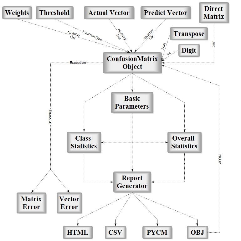
Fig1. ConfusionMatrix Block Diagram
Installation
Source code
- Download Version 2.1 or Latest Source
- Run
pip install -r requirements.txtorpip3 install -r requirements.txt(Need root access) - Run
python3 setup.py installorpython setup.py install(Need root access)
PyPI
- Check Python Packaging User Guide
- Run
pip install pycm==2.1orpip3 install pycm==2.1(Need root access)
Conda
- Check Conda Managing Package
conda install -c sepandhaghighi pycm(Need root access)
Easy install
- Run
easy_install --upgrade pycm(Need root access)
Usage
From vector
from pycm import *
y_actu = [2, 0, 2, 2, 0, 1, 1, 2, 2, 0, 1, 2]
y_pred = [0, 0, 2, 1, 0, 2, 1, 0, 2, 0, 2, 2]
cm = ConfusionMatrix(y_actu, y_pred,digit=5)
- Notice : `digit` (the number of digits to the right of the decimal point in a number) is new in version 0.6 (default value : 5)
- Only for print and save
cm
pycm.ConfusionMatrix(classes: [0, 1, 2])
cm.actual_vector
[2, 0, 2, 2, 0, 1, 1, 2, 2, 0, 1, 2]
cm.predict_vector
[0, 0, 2, 1, 0, 2, 1, 0, 2, 0, 2, 2]
cm.classes
[0, 1, 2]
cm.class_stat
{'ACC': {0: 0.8333333333333334, 1: 0.75, 2: 0.5833333333333334},
 'AGM': {0: 0.837285964012303, 1: 0.6919986974962765, 2: 0.6071224016819726},
 'AM': {0: 2, 1: -1, 2: -1},
 'AUC': {0: 0.8888888888888888, 1: 0.611111111111111, 2: 0.5833333333333333},
 'AUCI': {0: 'Very Good', 1: 'Fair', 2: 'Poor'},
 'BCD': {0: 0.08333333333333333,
  1: 0.041666666666666664,
  2: 0.041666666666666664},
 'BM': {0: 0.7777777777777777, 1: 0.2222222222222221, 2: 0.16666666666666652},
 'CEN': {0: 0.25, 1: 0.49657842846620864, 2: 0.6044162769630221},
 'DOR': {0: 'None', 1: 3.999999999999998, 2: 1.9999999999999998},
 'DP': {0: 'None', 1: 0.331933069996499, 2: 0.16596653499824957},
 'DPI': {0: 'None', 1: 'Poor', 2: 'Poor'},
 'ERR': {0: 0.16666666666666663, 1: 0.25, 2: 0.41666666666666663},
 'F0.5': {0: 0.6521739130434783,
  1: 0.45454545454545453,
  2: 0.5769230769230769},
 'F1': {0: 0.75, 1: 0.4, 2: 0.5454545454545454},
 'F2': {0: 0.8823529411764706, 1: 0.35714285714285715, 2: 0.5172413793103449},
 'FDR': {0: 0.4, 1: 0.5, 2: 0.4},
 'FN': {0: 0, 1: 2, 2: 3},
 'FNR': {0: 0.0, 1: 0.6666666666666667, 2: 0.5},
 'FOR': {0: 0.0, 1: 0.19999999999999996, 2: 0.4285714285714286},
 'FP': {0: 2, 1: 1, 2: 2},
 'FPR': {0: 0.2222222222222222,
  1: 0.11111111111111116,
  2: 0.33333333333333337},
 'G': {0: 0.7745966692414834, 1: 0.408248290463863, 2: 0.5477225575051661},
 'GI': {0: 0.7777777777777777, 1: 0.2222222222222221, 2: 0.16666666666666652},
 'GM': {0: 0.8819171036881969, 1: 0.5443310539518174, 2: 0.5773502691896257},
 'IBA': {0: 0.9506172839506174, 1: 0.1316872427983539, 2: 0.2777777777777778},
 'IS': {0: 1.263034405833794, 1: 1.0, 2: 0.2630344058337938},
 'J': {0: 0.6, 1: 0.25, 2: 0.375},
 'LS': {0: 2.4, 1: 2.0, 2: 1.2},
 'MCC': {0: 0.6831300510639732, 1: 0.25819888974716115, 2: 0.1690308509457033},
 'MCEN': {0: 0.2643856189774724, 1: 0.5, 2: 0.6875},
 'MK': {0: 0.6000000000000001, 1: 0.30000000000000004, 2: 0.17142857142857126},
 'N': {0: 9, 1: 9, 2: 6},
 'NLR': {0: 0.0, 1: 0.7500000000000001, 2: 0.75},
 'NPV': {0: 1.0, 1: 0.8, 2: 0.5714285714285714},
 'OP': {0: 0.7083333333333334, 1: 0.2954545454545454, 2: 0.4404761904761905},
 'P': {0: 3, 1: 3, 2: 6},
 'PLR': {0: 4.5, 1: 2.9999999999999987, 2: 1.4999999999999998},
 'PLRI': {0: 'Poor', 1: 'Poor', 2: 'Poor'},
 'POP': {0: 12, 1: 12, 2: 12},
 'PPV': {0: 0.6, 1: 0.5, 2: 0.6},
 'PRE': {0: 0.25, 1: 0.25, 2: 0.5},
 'Q': {0: 'None', 1: 0.6, 2: 0.3333333333333333},
 'RACC': {0: 0.10416666666666667,
  1: 0.041666666666666664,
  2: 0.20833333333333334},
 'RACCU': {0: 0.1111111111111111,
  1: 0.04340277777777778,
  2: 0.21006944444444442},
 'TN': {0: 7, 1: 8, 2: 4},
 'TNR': {0: 0.7777777777777778, 1: 0.8888888888888888, 2: 0.6666666666666666},
 'TON': {0: 7, 1: 10, 2: 7},
 'TOP': {0: 5, 1: 2, 2: 5},
 'TP': {0: 3, 1: 1, 2: 3},
 'TPR': {0: 1.0, 1: 0.3333333333333333, 2: 0.5},
 'Y': {0: 0.7777777777777777, 1: 0.2222222222222221, 2: 0.16666666666666652},
 'dInd': {0: 0.2222222222222222, 1: 0.6758625033664689, 2: 0.6009252125773316},
 'sInd': {0: 0.8428651597363228, 1: 0.5220930407198541, 2: 0.5750817072006014}}
- Notice : `cm.statistic_result` prev versions (0.2 >)
cm.overall_stat
{'95% CI': (0.30438856248221097, 0.8622781041844558),
 'AUNP': 0.6666666666666666,
 'AUNU': 0.6944444444444443,
 'Bennett S': 0.37500000000000006,
 'CBA': 0.4777777777777778,
 'Chi-Squared': 6.6,
 'Chi-Squared DF': 4,
 'Conditional Entropy': 0.9591479170272448,
 'Cramer V': 0.5244044240850757,
 'Cross Entropy': 1.5935164295556343,
 'Gwet AC1': 0.3893129770992367,
 'Hamming Loss': 0.41666666666666663,
 'Joint Entropy': 2.4591479170272446,
 'KL Divergence': 0.09351642955563438,
 'Kappa': 0.35483870967741943,
 'Kappa 95% CI': (-0.07707577422109269, 0.7867531935759315),
 'Kappa No Prevalence': 0.16666666666666674,
 'Kappa Standard Error': 0.2203645326012817,
 'Kappa Unbiased': 0.34426229508196726,
 'Lambda A': 0.16666666666666666,
 'Lambda B': 0.42857142857142855,
 'Mutual Information': 0.5242078379544426,
 'NIR': 0.5,
 'Overall ACC': 0.5833333333333334,
 'Overall CEN': 0.4638112995385119,
 'Overall J': (1.225, 0.4083333333333334),
 'Overall MCC': 0.36666666666666664,
 'Overall MCEN': 0.5189369467580801,
 'Overall RACC': 0.3541666666666667,
 'Overall RACCU': 0.3645833333333333,
 'P-Value': 0.38720703125,
 'PPV Macro': 0.5666666666666668,
 'PPV Micro': 0.5833333333333334,
 'Pearson C': 0.5956833971812705,
 'Phi-Squared': 0.5499999999999999,
 'RCI': 0.3494718919696284,
 'RR': 4.0,
 'Reference Entropy': 1.5,
 'Response Entropy': 1.4833557549816874,
 'SOA1(Landis & Koch)': 'Fair',
 'SOA2(Fleiss)': 'Poor',
 'SOA3(Altman)': 'Fair',
 'SOA4(Cicchetti)': 'Poor',
 'Scott PI': 0.34426229508196726,
 'Standard Error': 0.14231876063832777,
 'TPR Macro': 0.611111111111111,
 'TPR Micro': 0.5833333333333334,
 'Zero-one Loss': 5}
- Notice : new in version 0.3
- Notice : `_` removed from overall statistics names in version 1.6
cm.table
{0: {0: 3, 1: 0, 2: 0}, 1: {0: 0, 1: 1, 2: 2}, 2: {0: 2, 1: 1, 2: 3}}
cm.matrix
{0: {0: 3, 1: 0, 2: 0}, 1: {0: 0, 1: 1, 2: 2}, 2: {0: 2, 1: 1, 2: 3}}
cm.normalized_matrix
{0: {0: 1.0, 1: 0.0, 2: 0.0},
 1: {0: 0.0, 1: 0.33333, 2: 0.66667},
 2: {0: 0.33333, 1: 0.16667, 2: 0.5}}
cm.normalized_table
{0: {0: 1.0, 1: 0.0, 2: 0.0},
 1: {0: 0.0, 1: 0.33333, 2: 0.66667},
 2: {0: 0.33333, 1: 0.16667, 2: 0.5}}
- Notice : `matrix`, `normalized_matrix` & `normalized_table` added in version 1.5 (changed from print style)
import numpy
y_actu = numpy.array([2, 0, 2, 2, 0, 1, 1, 2, 2, 0, 1, 2])
y_pred = numpy.array([0, 0, 2, 1, 0, 2, 1, 0, 2, 0, 2, 2])
cm = ConfusionMatrix(y_actu, y_pred,digit=5)
cm
pycm.ConfusionMatrix(classes: [0, 1, 2])
- Notice : `numpy.array` support in versions > 0.7
Direct CM
cm2 = ConfusionMatrix(matrix={0: {0: 3, 1: 0, 2: 0}, 1: {0: 0, 1: 1, 2: 2}, 2: {0: 2, 1: 1, 2: 3}},digit=5)
cm2
pycm.ConfusionMatrix(classes: [0, 1, 2])
cm2.actual_vector
cm2.predict_vector
cm2.classes
[0, 1, 2]
cm2.class_stat
{'ACC': {0: 0.8333333333333334, 1: 0.75, 2: 0.5833333333333334},
 'AGM': {0: 0.837285964012303, 1: 0.6919986974962765, 2: 0.6071224016819726},
 'AM': {0: 2, 1: -1, 2: -1},
 'AUC': {0: 0.8888888888888888, 1: 0.611111111111111, 2: 0.5833333333333333},
 'AUCI': {0: 'Very Good', 1: 'Fair', 2: 'Poor'},
 'BCD': {0: 0.08333333333333333,
  1: 0.041666666666666664,
  2: 0.041666666666666664},
 'BM': {0: 0.7777777777777777, 1: 0.2222222222222221, 2: 0.16666666666666652},
 'CEN': {0: 0.25, 1: 0.49657842846620864, 2: 0.6044162769630221},
 'DOR': {0: 'None', 1: 3.999999999999998, 2: 1.9999999999999998},
 'DP': {0: 'None', 1: 0.331933069996499, 2: 0.16596653499824957},
 'DPI': {0: 'None', 1: 'Poor', 2: 'Poor'},
 'ERR': {0: 0.16666666666666663, 1: 0.25, 2: 0.41666666666666663},
 'F0.5': {0: 0.6521739130434783,
  1: 0.45454545454545453,
  2: 0.5769230769230769},
 'F1': {0: 0.75, 1: 0.4, 2: 0.5454545454545454},
 'F2': {0: 0.8823529411764706, 1: 0.35714285714285715, 2: 0.5172413793103449},
 'FDR': {0: 0.4, 1: 0.5, 2: 0.4},
 'FN': {0: 0, 1: 2, 2: 3},
 'FNR': {0: 0.0, 1: 0.6666666666666667, 2: 0.5},
 'FOR': {0: 0.0, 1: 0.19999999999999996, 2: 0.4285714285714286},
 'FP': {0: 2, 1: 1, 2: 2},
 'FPR': {0: 0.2222222222222222,
  1: 0.11111111111111116,
  2: 0.33333333333333337},
 'G': {0: 0.7745966692414834, 1: 0.408248290463863, 2: 0.5477225575051661},
 'GI': {0: 0.7777777777777777, 1: 0.2222222222222221, 2: 0.16666666666666652},
 'GM': {0: 0.8819171036881969, 1: 0.5443310539518174, 2: 0.5773502691896257},
 'IBA': {0: 0.9506172839506174, 1: 0.1316872427983539, 2: 0.2777777777777778},
 'IS': {0: 1.263034405833794, 1: 1.0, 2: 0.2630344058337938},
 'J': {0: 0.6, 1: 0.25, 2: 0.375},
 'LS': {0: 2.4, 1: 2.0, 2: 1.2},
 'MCC': {0: 0.6831300510639732, 1: 0.25819888974716115, 2: 0.1690308509457033},
 'MCEN': {0: 0.2643856189774724, 1: 0.5, 2: 0.6875},
 'MK': {0: 0.6000000000000001, 1: 0.30000000000000004, 2: 0.17142857142857126},
 'N': {0: 9, 1: 9, 2: 6},
 'NLR': {0: 0.0, 1: 0.7500000000000001, 2: 0.75},
 'NPV': {0: 1.0, 1: 0.8, 2: 0.5714285714285714},
 'OP': {0: 0.7083333333333334, 1: 0.2954545454545454, 2: 0.4404761904761905},
 'P': {0: 3, 1: 3, 2: 6},
 'PLR': {0: 4.5, 1: 2.9999999999999987, 2: 1.4999999999999998},
 'PLRI': {0: 'Poor', 1: 'Poor', 2: 'Poor'},
 'POP': {0: 12, 1: 12, 2: 12},
 'PPV': {0: 0.6, 1: 0.5, 2: 0.6},
 'PRE': {0: 0.25, 1: 0.25, 2: 0.5},
 'Q': {0: 'None', 1: 0.6, 2: 0.3333333333333333},
 'RACC': {0: 0.10416666666666667,
  1: 0.041666666666666664,
  2: 0.20833333333333334},
 'RACCU': {0: 0.1111111111111111,
  1: 0.04340277777777778,
  2: 0.21006944444444442},
 'TN': {0: 7, 1: 8, 2: 4},
 'TNR': {0: 0.7777777777777778, 1: 0.8888888888888888, 2: 0.6666666666666666},
 'TON': {0: 7, 1: 10, 2: 7},
 'TOP': {0: 5, 1: 2, 2: 5},
 'TP': {0: 3, 1: 1, 2: 3},
 'TPR': {0: 1.0, 1: 0.3333333333333333, 2: 0.5},
 'Y': {0: 0.7777777777777777, 1: 0.2222222222222221, 2: 0.16666666666666652},
 'dInd': {0: 0.2222222222222222, 1: 0.6758625033664689, 2: 0.6009252125773316},
 'sInd': {0: 0.8428651597363228, 1: 0.5220930407198541, 2: 0.5750817072006014}}
cm2.overall_stat
{'95% CI': (0.30438856248221097, 0.8622781041844558),
 'AUNP': 0.6666666666666666,
 'AUNU': 0.6944444444444443,
 'Bennett S': 0.37500000000000006,
 'CBA': 0.4777777777777778,
 'Chi-Squared': 6.6,
 'Chi-Squared DF': 4,
 'Conditional Entropy': 0.9591479170272448,
 'Cramer V': 0.5244044240850757,
 'Cross Entropy': 1.5935164295556343,
 'Gwet AC1': 0.3893129770992367,
 'Hamming Loss': 0.41666666666666663,
 'Joint Entropy': 2.4591479170272446,
 'KL Divergence': 0.09351642955563438,
 'Kappa': 0.35483870967741943,
 'Kappa 95% CI': (-0.07707577422109269, 0.7867531935759315),
 'Kappa No Prevalence': 0.16666666666666674,
 'Kappa Standard Error': 0.2203645326012817,
 'Kappa Unbiased': 0.34426229508196726,
 'Lambda A': 0.16666666666666666,
 'Lambda B': 0.42857142857142855,
 'Mutual Information': 0.5242078379544426,
 'NIR': 0.5,
 'Overall ACC': 0.5833333333333334,
 'Overall CEN': 0.4638112995385119,
 'Overall J': (1.225, 0.4083333333333334),
 'Overall MCC': 0.36666666666666664,
 'Overall MCEN': 0.5189369467580801,
 'Overall RACC': 0.3541666666666667,
 'Overall RACCU': 0.3645833333333333,
 'P-Value': 0.38720703125,
 'PPV Macro': 0.5666666666666668,
 'PPV Micro': 0.5833333333333334,
 'Pearson C': 0.5956833971812705,
 'Phi-Squared': 0.5499999999999999,
 'RCI': 0.3494718919696284,
 'RR': 4.0,
 'Reference Entropy': 1.5,
 'Response Entropy': 1.4833557549816874,
 'SOA1(Landis & Koch)': 'Fair',
 'SOA2(Fleiss)': 'Poor',
 'SOA3(Altman)': 'Fair',
 'SOA4(Cicchetti)': 'Poor',
 'Scott PI': 0.34426229508196726,
 'Standard Error': 0.14231876063832777,
 'TPR Macro': 0.611111111111111,
 'TPR Micro': 0.5833333333333334,
 'Zero-one Loss': 5}
- Notice : new in version 0.8.1
- In direct matrix mode `actual_vector` and `predict_vector` are empty
Activation threshold
threshold is added in version 0.9 for real value prediction.
For more information visit Example 3
- Notice : new in version 0.9
Load from file
file is added in version 0.9.5 in order to load saved confusion matrix with .obj format generated by save_obj method.
For more information visit Example 4
- Notice : new in version 0.9.5
Sample weights
sample_weight is added in version 1.2
For more information visit Example 5
- Notice : new in version 1.2
Transpose
transpose is added in version 1.2 in order to transpose input matrix (only in Direct CM mode)
cm = ConfusionMatrix(matrix={0: {0: 3, 1: 0, 2: 0}, 1: {0: 0, 1: 1, 2: 2}, 2: {0: 2, 1: 1, 2: 3}},digit=5,transpose=True)
cm.print_matrix()
Predict 0       1       2
Actual
0       3       0       2

1       0       1       1

2       0       2       3
- Notice : new in version 1.2
Relabel
relabel method is added in version 1.5 in order to change ConfusionMatrix classnames.
cm.relabel(mapping={0:"L1",1:"L2",2:"L3"})
cm
pycm.ConfusionMatrix(classes: ['L1', 'L2', 'L3'])
- Notice : new in version 1.5
Online help
online_help function is added in version 1.1 in order to open each statistics definition in web browser
>>> from pycm import online_help
>>> online_help("J")
>>> online_help("SOA1(Landis & Koch)")
>>> online_help(2)
- List of items are available by calling
online_help()(without argument)
online_help()
Please choose one parameter :

Example : online_help("J") or online_help(2)

1-95% CI
2-ACC
3-AGM
4-AM
5-AUC
6-AUCI
7-AUNP
8-AUNU
9-BCD
10-BM
11-Bennett S
12-CBA
13-CEN
14-Chi-Squared
15-Chi-Squared DF
16-Conditional Entropy
17-Cramer V
18-Cross Entropy
19-DOR
20-DP
21-DPI
22-ERR
23-F0.5
24-F1
25-F2
26-FDR
27-FN
28-FNR
29-FOR
30-FP
31-FPR
32-G
33-GI
34-GM
35-Gwet AC1
36-Hamming Loss
37-IBA
38-IS
39-J
40-Joint Entropy
41-KL Divergence
42-Kappa
43-Kappa 95% CI
44-Kappa No Prevalence
45-Kappa Standard Error
46-Kappa Unbiased
47-LS
48-Lambda A
49-Lambda B
50-MCC
51-MCEN
52-MK
53-Mutual Information
54-N
55-NIR
56-NLR
57-NPV
58-OP
59-Overall ACC
60-Overall CEN
61-Overall J
62-Overall MCC
63-Overall MCEN
64-Overall RACC
65-Overall RACCU
66-P
67-P-Value
68-PLR
69-PLRI
70-POP
71-PPV
72-PPV Macro
73-PPV Micro
74-PRE
75-Pearson C
76-Phi-Squared
77-Q
78-RACC
79-RACCU
80-RCI
81-RR
82-Reference Entropy
83-Response Entropy
84-SOA1(Landis & Koch)
85-SOA2(Fleiss)
86-SOA3(Altman)
87-SOA4(Cicchetti)
88-Scott PI
89-Standard Error
90-TN
91-TNR
92-TON
93-TOP
94-TP
95-TPR
96-TPR Macro
97-TPR Micro
98-Y
99-Zero-one Loss
100-dInd
101-sInd
Parameter recommender
This option has been added in version 1.9 in order to recommend most related parameters considering the characteristics of the input dataset. The characteristics according to which the parameters are suggested are balance/imbalance and binary/multiclass. All suggestions can be categorized into three main groups: imbalanced dataset, binary classification for a balanced dataset, and multi-class classification for a balanced dataset. The recommendation lists have been gathered according to the respective paper of each parameter and the capabilities which had been claimed by the paper.
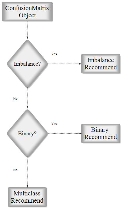
Fig2. Parameter Recommender Block Diagram
cm.imbalance
False
cm.binary
False
cm.recommended_list
['ERR',
 'TPR Micro',
 'TPR Macro',
 'PPV Micro',
 'PPV Macro',
 'ACC',
 'Overall ACC',
 'MCC',
 'Overall MCC',
 'BCD',
 'Hamming Loss',
 'Zero-one Loss']
- Notice : also available in HTML report
- Notice : The recommender system assumes that the input is the result of classification over the whole data rather than just a part of it. If the confusion matrix is the result of test data classification, the recommendation is not valid.
Comapre
In version 2.0 a method for comparing several confusion matrices is introduced. This option is a combination of several overall and class-based benchmarks. Each of the benchmarks evaluates the performance of the classification algorithm from good to poor and give them a numeric score. The score of good performance is 1 and for the poor performance is 0.
After that, two scores are calculated for each confusion matrices, overall and class based. The overall score is the average of the score of four overall benchmarks which are Landis & Koch, Fleiss, Altman, and Cicchetti. And with a same manner, the class based score is the average of the score of three class-based benchmarks which are Positive Likelihood Ratio Interpretation, Discriminant Power Interpretation, and AUC value Interpretation. It should be notice that if one of the benchmarks returns none for one of the classes, that benchmarks will be eliminate in total averaging. If user set weights for the classes, the averaging over the value of class-based benchmark scores will transform to a weighted average.
If the user set the value of by_class boolean input True, the best confusion matrix is the one with the maximum class-based score. Otherwise, if a confusion matrix obtain the maximum of the both overall and class-based score, that will be the reported as the best confusion matrix but in any other cases the compare object doesn’t select best confusion matrix.

Fig3. Compare Block Diagram
cm2 = ConfusionMatrix(matrix={0:{0:2,1:50,2:6},1:{0:5,1:50,2:3},2:{0:1,1:7,2:50}})
cm3 = ConfusionMatrix(matrix={0:{0:50,1:2,2:6},1:{0:50,1:5,2:3},2:{0:1,1:55,2:2}})
cp = Compare({"cm2":cm2,"cm3":cm3})
print(cp)
Best : cm2

Rank  Name   Class-Score    Overall-Score
1     cm2    4.15           1.48333
2     cm3    2.75           0.95
cp.scores
{'cm2': {'class': 4.15, 'overall': 1.48333},
 'cm3': {'class': 2.75, 'overall': 0.95}}
cp.sorted
['cm2', 'cm3']
cp.best
pycm.ConfusionMatrix(classes: [0, 1, 2])
cp.best_name
'cm2'
cp2 = Compare({"cm2":cm2,"cm3":cm3},by_class=True,weight={0:5,1:1,2:1})
print(cp2)
Best : cm3

Rank  Name   Class-Score    Overall-Score
1     cm3    8.15           0.95
2     cm2    6.95           1.48333
Acceptable data types
ConfusionMatrix
actual_vector: pythonlistor numpyarrayof any stringable objectspredict_vector: pythonlistor numpyarrayof any stringable objectsmatrix:dictdigit:intthreshold:FunctionType (function or lambda)file:File objectsample_weight: pythonlistor numpyarrayof numberstranspose:bool
- run
help(ConfusionMatrix)for more information
Compare
cm_dict: pythondictofConfusionMatrixobject (str:ConfusionMatrix)by_class:boolweight: pythondictof class weights (class_name:float)digit:int
- run
help(Compare)for more information
Basic parameters
TP (True positive)
A true positive test result is one that detects the condition when the condition is present (correctly identified) [3].
cm.TP
{'L1': 3, 'L2': 1, 'L3': 3}
TN (True negative)
A true negative test result is one that does not detect the condition when the condition is absent correctly rejected) [3].
cm.TN
{'L1': 7, 'L2': 8, 'L3': 4}
FP (False positive)
A false positive test result is one that detects the condition when the condition is absent (incorrectly identified) [3].
cm.FP
{'L1': 0, 'L2': 2, 'L3': 3}
FN (False negative)
A false negative test result is one that does not detect the condition when the condition is present (incorrectly rejected) [3].
cm.FN
{'L1': 2, 'L2': 1, 'L3': 2}
P (Condition positive)
Number of positive samples. Also known as support (the number of occurrences of each class in y_true) [3].
cm.P
{'L1': 5, 'L2': 2, 'L3': 5}
N (Condition negative)
Number of negative samples [3].
cm.N
{'L1': 7, 'L2': 10, 'L3': 7}
TOP (Test outcome positive)
Number of positive outcomes [3].
cm.TOP
{'L1': 3, 'L2': 3, 'L3': 6}
TON (Test outcome negative)
Number of negative outcomes [3].
cm.TON
{'L1': 9, 'L2': 9, 'L3': 6}
POP (Population)
For more information visit [3].
cm.POP
{'L1': 12, 'L2': 12, 'L3': 12}
Class statistics
TPR (True positive rate)
Sensitivity (also called the true positive rate, the recall, or probability of detection in some fields) measures the proportion of positives that are correctly identified as such (e.g. the percentage of sick people who are correctly identified as having the condition) [3].
cm.TPR
{'L1': 0.6, 'L2': 0.5, 'L3': 0.6}
TNR (True negative rate)
Specificity (also called the true negative rate) measures the proportion of negatives that are correctly identified as such (e.g. the percentage of healthy people who are correctly identified as not having the condition) [3].
cm.TNR
{'L1': 1.0, 'L2': 0.8, 'L3': 0.5714285714285714}
PPV (Positive predictive value)
Predictive value positive is the proportion of positives that correspond to the presence of the condition [3].
cm.PPV
{'L1': 1.0, 'L2': 0.3333333333333333, 'L3': 0.5}
NPV (Negative predictive value)
Predictive value negative is the proportion of negatives that correspond to the absence of the condition [3].
cm.NPV
{'L1': 0.7777777777777778, 'L2': 0.8888888888888888, 'L3': 0.6666666666666666}
FNR (False negative rate)
The false negative rate is the proportion of positives which yield negative test outcomes with the test, i.e., the conditional probability of a negative test result given that the condition being looked for is present [3].
cm.FNR
{'L1': 0.4, 'L2': 0.5, 'L3': 0.4}
FPR (False positive rate)
The false positive rate is the proportion of all negatives that still yield positive test outcomes, i.e., the conditional probability of a positive test result given an event that was not present [3].
The false positive rate is equal to the significance level. The specificity of the test is equal to 1 minus the false positive rate.
cm.FPR
{'L1': 0.0, 'L2': 0.19999999999999996, 'L3': 0.4285714285714286}
FDR (False discovery rate)
The false discovery rate (FDR) is a method of conceptualizing the rate of type I errors in null hypothesis testing when conducting multiple comparisons. FDR-controlling procedures are designed to control the expected proportion of "discoveries" (rejected null hypotheses) that are false (incorrect rejections) [3].
cm.FDR
{'L1': 0.0, 'L2': 0.6666666666666667, 'L3': 0.5}
FOR (False omission rate)
False omission rate (FOR) is a statistical method used in multiple hypothesis testing to correct for multiple comparisons and it is the complement of the negative predictive value. It measures the proportion of false negatives which are incorrectly rejected [3].
cm.FOR
{'L1': 0.2222222222222222,
 'L2': 0.11111111111111116,
 'L3': 0.33333333333333337}
ACC (Accuracy)
The accuracy is the number of correct predictions from all predictions made [3].
cm.ACC
{'L1': 0.8333333333333334, 'L2': 0.75, 'L3': 0.5833333333333334}
ERR (Error rate)
The accuracy is the number of incorrect predictions from all predictions made [3].
cm.ERR
{'L1': 0.16666666666666663, 'L2': 0.25, 'L3': 0.41666666666666663}
- Notice : new in version 0.4
FBeta-Score
In statistical analysis of classification, the F1 score (also F-score or F-measure) is a measure of a test's accuracy. It considers both the precision p and the recall r of the test to compute the score. The F1 score is the harmonic average of the precision and recall, where F1 score reaches its best value at 1 (perfect precision and recall) and worst at 0 [3].
cm.F1
{'L1': 0.75, 'L2': 0.4, 'L3': 0.5454545454545454}
cm.F05
{'L1': 0.8823529411764706, 'L2': 0.35714285714285715, 'L3': 0.5172413793103449}
cm.F2
{'L1': 0.6521739130434783, 'L2': 0.45454545454545453, 'L3': 0.5769230769230769}
cm.F_beta(beta=4)
{'L1': 0.6144578313253012, 'L2': 0.4857142857142857, 'L3': 0.5930232558139535}
- Notice : new in version 0.4
MCC (Matthews correlation coefficient)
The Matthews correlation coefficient is used in machine learning as a measure of the quality of binary (two-class) classifications, introduced by biochemist Brian W. Matthews in 1975. It takes into account true and false positives and negatives and is generally regarded as a balanced measure which can be used even if the classes are of very different sizes.The MCC is in essence a correlation coefficient between the observed and predicted binary classifications; it returns a value between −1 and +1. A coefficient of +1 represents a perfect prediction, 0 no better than random prediction and −1 indicates total disagreement between prediction and observation [27].
cm.MCC
{'L1': 0.6831300510639732, 'L2': 0.25819888974716115, 'L3': 0.1690308509457033}
BM (Bookmaker informedness)
The informedness of a prediction method as captured by a contingency matrix is defined as the probability that the prediction method will make a correct decision as opposed to guessing and is calculated using the bookmaker algorithm [2].
cm.BM
{'L1': 0.6000000000000001,
 'L2': 0.30000000000000004,
 'L3': 0.17142857142857126}
MK (Markedness)
In statistics and psychology, the social science concept of markedness is quantified as a measure of how much one variable is marked as a predictor or possible cause of another, and is also known as Δp (deltaP) in simple two-choice cases [2].
cm.MK
{'L1': 0.7777777777777777, 'L2': 0.2222222222222221, 'L3': 0.16666666666666652}
PLR (Positive likelihood ratio)
Likelihood ratios are used for assessing the value of performing a diagnostic test. They use the sensitivity and specificity of the test to determine whether a test result usefully changes the probability that a condition (such as a disease state) exists. The first description of the use of likelihood ratios for decision rules was made at a symposium on information theory in 1954 [28].
cm.PLR
{'L1': 'None', 'L2': 2.5000000000000004, 'L3': 1.4}
- Notice : `LR+` renamed to `PLR` in version 1.5
NLR (Negative likelihood ratio)
Likelihood ratios are used for assessing the value of performing a diagnostic test. They use the sensitivity and specificity of the test to determine whether a test result usefully changes the probability that a condition (such as a disease state) exists. The first description of the use of likelihood ratios for decision rules was made at a symposium on information theory in 1954 [28].
cm.NLR
{'L1': 0.4, 'L2': 0.625, 'L3': 0.7000000000000001}
- Notice : `LR-` renamed to `NLR` in version 1.5
DOR (Diagnostic odds ratio)
The diagnostic odds ratio is a measure of the effectiveness of a diagnostic test. It is defined as the ratio of the odds of the test being positive if the subject has a disease relative to the odds of the test being positive if the subject does not have the disease [28].
cm.DOR
{'L1': 'None', 'L2': 4.000000000000001, 'L3': 1.9999999999999998}
PRE (Prevalence)
Prevalence is a statistical concept referring to the number of cases of a disease that are present in a particular population at a given time (Reference Likelihood) [14].
cm.PRE
{'L1': 0.4166666666666667, 'L2': 0.16666666666666666, 'L3': 0.4166666666666667}
G (G-measure)
Geometric mean of precision and sensitivity, also known as Fowlkes–Mallows index [3].
cm.G
{'L1': 0.7745966692414834, 'L2': 0.408248290463863, 'L3': 0.5477225575051661}
RACC (Random accuracy)
The expected accuracy from a strategy of randomly guessing categories according to reference and response distributions [24].
cm.RACC
{'L1': 0.10416666666666667,
 'L2': 0.041666666666666664,
 'L3': 0.20833333333333334}
- Notice : new in version 0.3
RACCU (Random accuracy unbiased)
The expected accuracy from a strategy of randomly guessing categories according to the average of the reference and response distributions [25].
cm.RACCU
{'L1': 0.1111111111111111,
 'L2': 0.04340277777777778,
 'L3': 0.21006944444444442}
- Notice : new in version 0.8.1
J (Jaccard index)
The Jaccard index, also known as Intersection over Union and the Jaccard similarity coefficient (originally coined coefficient de communauté by Paul Jaccard), is a statistic used for comparing the similarity and diversity of sample sets [29].
cm.J
{'L1': 0.6, 'L2': 0.25, 'L3': 0.375}
- Notice : new in version 0.9
IS (Information score)
cm.IS
{'L1': 1.2630344058337937, 'L2': 0.9999999999999998, 'L3': 0.26303440583379367}
- Notice : new in version 1.3
CEN (Confusion entropy)
CEN based upon the concept of entropy for evaluating classifier performances. By exploiting the misclassification information of confusion matrices, the measure evaluates the confusion level of the class distribution of misclassified samples. Both theoretical analysis and statistical results show that the proposed measure is more discriminating than accuracy and RCI while it remains relatively consistent with the two measures. Moreover, it is more capable of measuring how the samples of different classes have been separated from each other. Hence the proposed measure is more precise than the two measures and can substitute for them to evaluate classifiers in classification applications [17].
cm.CEN
{'L1': 0.25, 'L2': 0.49657842846620864, 'L3': 0.6044162769630221}
- Notice : new in version 1.3
MCEN (Modified confusion entropy)
Modified version of CEN [19].
cm.MCEN
{'L1': 0.2643856189774724, 'L2': 0.5, 'L3': 0.6875}
- Notice : new in version 1.3
AUC (Area under the ROC curve)
Thus, AUC corresponds to the arithmetic mean of sensitivity and specificity values of each class [23].
cm.AUC
{'L1': 0.8, 'L2': 0.65, 'L3': 0.5857142857142856}
- Notice : new in version 1.4
- Notice : this is an approximate calculation of AUC
dInd (Distance index)
Euclidean distance of a ROC point from the top left corner of the ROC space, which can take values between 0 (perfect classification) and sqrt(2) [23].
cm.dInd
{'L1': 0.4, 'L2': 0.5385164807134504, 'L3': 0.5862367008195198}
- Notice : new in version 1.4
sInd (Similarity index)
sInd is comprised between 0 (no correct classifications) and 1 (perfect classification) [23].
cm.sInd
{'L1': 0.717157287525381, 'L2': 0.6192113447068046, 'L3': 0.5854680534700882}
- Notice : new in version 1.4
DP (Discriminant power)
Discriminant power (DP) is a measure that summarizes sensitivity and specificity. The DP has been used mainly in feature selection over imbalanced data [33].
cm.DP
{'L1': 'None', 'L2': 0.33193306999649924, 'L3': 0.1659665349982495}
- Notice : new in version 1.5
Y (Youden index)
Youden’s index, evaluates the algorithm’s ability to avoid failure; it’s derived from sensitivity and specificity and denotes a linear correspondence balanced accuracy. As Youden’s index is a linear transformation of the mean sensitivity and specificity, its values are difficult to interpret, we retain that a higher value of Y indicates better ability to avoid failure. Youden’s index has been conventionally used to evaluate tests diagnostic, improve efficiency of Telemedical prevention [33] [34].
cm.Y
{'L1': 0.6000000000000001,
 'L2': 0.30000000000000004,
 'L3': 0.17142857142857126}
- Notice : new in version 1.5
PLRI (Positive likelihood ratio interpretation)
For more information visit [33].
| PLR | Model contribution |
| 1 > | Negligible |
| 1 - 5 | Poor |
| 5 - 10 | Fair |
| > 10 | Good |
cm.PLRI
{'L1': 'None', 'L2': 'Poor', 'L3': 'Poor'}
- Notice : new in version 1.5
DPI (Discriminant power interpretation)
For more information visit [33].
| DP | Model contribution |
| 1 > | Poor |
| 1 - 2 | Limited |
| 2 - 3 | Fair |
| > 3 | Good |
cm.DPI
{'L1': 'None', 'L2': 'Poor', 'L3': 'Poor'}
- Notice : new in version 1.5
AUCI (AUC value interpretation)
For more information visit [33].
| AUC | Model performance |
| 0.5 - 0.6 | Poor |
| 0.6 - 0.7 | Fair |
| 0.7 - 0.8 | Good |
| 0.8 - 0.9 | Very Good |
| 0.9 - 1.0 | Excellent |
cm.AUCI
{'L1': 'Very Good', 'L2': 'Fair', 'L3': 'Poor'}
- Notice : new in version 1.6
GI (Gini index)
A chance-standardized variant of the AUC is given by Gini coefficient, taking values between 0 (no difference between the score distributions of the two classes) and 1 (complete separation between the two distributions). Gini coefficient is widespread use metric in imbalanced data learning [33].
cm.GI
{'L1': 0.6000000000000001,
 'L2': 0.30000000000000004,
 'L3': 0.17142857142857126}
- Notice : new in version 1.7
LS (Lift score)
cm.LS
{'L1': 2.4, 'L2': 2.0, 'L3': 1.2}
- Notice : new in version 1.8
AM (Automatic/Manual)
Difference between automatic and manual classification
cm.AM
{'L1': -2, 'L2': 1, 'L3': 1}
- Notice : new in version 1.9
BCD (Bray-Curtis dissimilarity)
In ecology and biology, the Bray–Curtis dissimilarity, named after J. Roger Bray and John T. Curtis, is a statistic used to quantify the compositional dissimilarity between two different sites, based on counts at each site [37].
cm.BCD
{'L1': 0.08333333333333333,
 'L2': 0.041666666666666664,
 'L3': 0.041666666666666664}
- Notice : new in version 1.9
OP (Optimized precision)
Optimized precision is a type of hybrid threshold metrics and has been proposed as a discriminator for building an optimized heuristic classifier. This metric is a combination of accuracy, sensitivity and specificity metrics. The sensitivity and specificity metric were used for stabilizing and optimizing the accuracy performance when dealing with imbalanced class of twoclass problems [40] [42].
cm.OP
{'L1': 0.5833333333333334, 'L2': 0.5192307692307692, 'L3': 0.5589430894308943}
- Notice : new in version 2.0
IBA (Index of balanced accuracy)
cm.IBA
{'L1': 0.36, 'L2': 0.27999999999999997, 'L3': 0.35265306122448975}
cm.IBA_alpha(0.5)
{'L1': 0.48, 'L2': 0.34, 'L3': 0.3477551020408163}
cm.IBA_alpha(0.1)
{'L1': 0.576, 'L2': 0.388, 'L3': 0.34383673469387754}
- Notice : new in version 2.0
GM (G-mean)
cm.GM
{'L1': 0.7745966692414834, 'L2': 0.6324555320336759, 'L3': 0.5855400437691198}
- Notice : new in version 2.0
Q (Yule's Q)
In statistics, Yule's Q, also known as the coefficient of colligation, is a measure of association between two binary variables [45].
cm.Q
{'L1': 'None', 'L2': 0.6, 'L3': 0.3333333333333333}
- Notice : new in version 2.1
AGM (Adjusted G-mean)
An adjusted version of geometric mean of specificity and sensitivity [46].
cm.AGM
{'L1': 0.8576400016262, 'L2': 0.708612108382005, 'L3': 0.5803410802752335}
- Notice : new in version 2.1
Overall statistics
Kappa
Kappa is a statistic which measures inter-rater agreement for qualitative (categorical) items. It is generally thought to be a more robust measure than simple percent agreement calculation, as kappa takes into account the possibility of the agreement occurring by chance [24].
cm.Kappa
0.35483870967741943
- Notice : new in version 0.3
Kappa unbiased
The unbiased kappa value is defined in terms of total accuracy and a slightly different computation of expected likelihood that averages the reference and response probabilities [25].
cm.KappaUnbiased
0.34426229508196726
- Notice : new in version 0.8.1
Kappa no prevalence
The kappa statistic adjusted for prevalence [14].
cm.KappaNoPrevalence
0.16666666666666674
- Notice : new in version 0.8.1
Kappa standard error
cm.Kappa_SE
0.2203645326012817
- Notice : new in version 0.7
Kappa 95% CI
cm.Kappa_CI
(-0.07707577422109269, 0.7867531935759315)
- Notice : new in version 0.7
Chi-squared
Pearson's chi-squared test is a statistical test applied to sets of categorical data to evaluate how likely it is that any observed difference between the sets arose by chance. It is suitable for unpaired data from large samples [10].
cm.Chi_Squared
6.6000000000000005
- Notice : new in version 0.7
Chi-squared DF
Number of degrees of freedom of this confusion matrix for the chi-squared statistic [10].
cm.DF
4
- Notice : new in version 0.7
Phi-squared
In statistics, the phi coefficient (or mean square contingency coefficient) is a measure of association for two binary variables. Introduced by Karl Pearson, this measure is similar to the Pearson correlation coefficient in its interpretation. In fact, a Pearson correlation coefficient estimated for two binary variables will return the phi coefficient [10].
cm.Phi_Squared
0.55
- Notice : new in version 0.7
Cramer's V
In statistics, Cramér's V (sometimes referred to as Cramér's phi) is a measure of association between two nominal variables, giving a value between 0 and +1 (inclusive). It is based on Pearson's chi-squared statistic and was published by Harald Cramér in 1946 [26].
cm.V
0.5244044240850758
- Notice : new in version 0.7
Standard error
The standard error (SE) of a statistic (usually an estimate of a parameter) is the standard deviation of its sampling distribution or an estimate of that standard deviation [31].
cm.SE
0.14231876063832777
- Notice : new in version 0.7
95% CI
In statistics, a confidence interval (CI) is a type of interval estimate (of a population parameter) that is computed from the observed data. The confidence level is the frequency (i.e., the proportion) of possible confidence intervals that contain the true value of their corresponding parameter. In other words, if confidence intervals are constructed using a given confidence level in an infinite number of independent experiments, the proportion of those intervals that contain the true value of the parameter will match the confidence level [31].
cm.CI
(0.30438856248221097, 0.8622781041844558)
- Notice : new in version 0.7
Bennett's S
Bennett, Alpert & Goldstein’s S is a statistical measure of inter-rater agreement. It was created by Bennett et al. in 1954. Bennett et al. suggested adjusting inter-rater reliability to accommodate the percentage of rater agreement that might be expected by chance was a better measure than simple agreement between raters [8].
cm.S
0.37500000000000006
- Notice : new in version 0.5
Scott's Pi
Scott's pi (named after William A. Scott) is a statistic for measuring inter-rater reliability for nominal data in communication studies. Textual entities are annotated with categories by different annotators, and various measures are used to assess the extent of agreement between the annotators, one of which is Scott's pi. Since automatically annotating text is a popular problem in natural language processing, and goal is to get the computer program that is being developed to agree with the humans in the annotations it creates, assessing the extent to which humans agree with each other is important for establishing a reasonable upper limit on computer performance [7].
cm.PI
0.34426229508196726
- Notice : new in version 0.5
Gwet's AC1
AC1 was originally introduced by Gwet in 2001 (Gwet, 2001). The interpretation of AC1 is similar to generalized kappa (Fleiss, 1971), which is used to assess interrater reliability of when there are multiple raters. Gwet (2002) demonstrated that AC1 can overcome the limitations that kappa is sensitive to trait prevalence and rater's classification probabilities (i.e., marginal probabilities), whereas AC1 provides more robust measure of interrater reliability [6].
cm.AC1
0.3893129770992367
- Notice : new in version 0.5
Reference entropy
The entropy of the decision problem itself as defined by the counts for the reference. The entropy of a distribution is the average negative log probability of outcomes [30].
cm.ReferenceEntropy
1.4833557549816874
- Notice : new in version 0.8.1
Response entropy
The entropy of the response distribution. The entropy of a distribution is the average negative log probability of outcomes [30].
cm.ResponseEntropy
1.5
- Notice : new in version 0.8.1
Cross entropy
The cross-entropy of the response distribution against the reference distribution. The cross-entropy is defined by the negative log probabilities of the response distribution weighted by the reference distribution [30].
cm.CrossEntropy
1.5833333333333335
- Notice : new in version 0.8.1
Joint entropy
The entropy of the joint reference and response distribution as defined by the underlying matrix [30].
cm.JointEntropy
2.4591479170272446
- Notice : new in version 0.8.1
Conditional entropy
The entropy of the distribution of categories in the response given that the reference category was as specified [30].
cm.ConditionalEntropy
0.9757921620455572
- Notice : new in version 0.8.1
Kullback-Liebler divergence
cm.KL
0.09997757835164581
- Notice : new in version 0.8.1
Mutual information
Mutual information is defined Kullback-Lieblier divergence, between the product of the individual distributions and the joint distribution. Mutual information is symmetric. We could also subtract the conditional entropy of the reference given the response from the reference entropy to get the same result [11] [30].
cm.MutualInformation
0.5242078379544428
- Notice : new in version 0.8.1
Goodman & Kruskal's lambda A
In probability theory and statistics, Goodman & Kruskal's lambda is a measure of proportional reduction in error in cross tabulation analysis [12].
cm.LambdaA
0.42857142857142855
- Notice : new in version 0.8.1
Goodman & Kruskal's lambda B
In probability theory and statistics, Goodman & Kruskal's lambda is a measure of proportional reduction in error in cross tabulation analysis [13].
cm.LambdaB
0.16666666666666666
- Notice : new in version 0.8.1
SOA1 (Landis & Koch's benchmark)
For more information visit [1].
| Kappa | Strength of Agreement |
| 0 > | Poor |
| 0 - 0.20 | Slight |
| 0.21 – 0.40 | Fair |
| 0.41 – 0.60 | Moderate |
| 0.61 – 0.80 | Substantial |
| 0.81 – 1.00 | Almost perfect |
cm.SOA1
'Fair'
- Notice : new in version 0.3
SOA2 (Fleiss' benchmark)
For more information visit [4].
| Kappa | Strength of Agreement |
| 0.40 > | Poor |
| 0.4 - 0.75 | Intermediate to Good |
| More than 0.75 | Excellent |
cm.SOA2
'Poor'
- Notice : new in version 0.4
SOA3 (Altman's benchmark)
For more information visit [5].
| Kappa | Strength of Agreement |
| 0.2 > | Poor |
| 0.21 – 0.40 | Fair |
| 0.41 – 0.60 | Moderate |
| 0.61 – 0.80 | Good |
| 0.81 – 1.00 | Very Good |
cm.SOA3
'Fair'
- Notice : new in version 0.4
SOA4 (Cicchetti's benchmark)
For more information visit [9].
| Kappa | Strength of Agreement |
| 0.4 > | Poor |
| 0.4 – 0.59 | Fair |
| 0.6 – 0.74 | Good |
| 0.74 – 1.00 | Excellent |
cm.SOA4
'Poor'
- Notice : new in version 0.7
Overall_ACC
For more information visit [3].
cm.Overall_ACC
0.5833333333333334
- Notice : new in version 0.4
Overall_RACC
For more information visit [24].
cm.Overall_RACC
0.3541666666666667
- Notice : new in version 0.4
Overall_RACCU
For more information visit [25].
cm.Overall_RACCU
0.3645833333333333
- Notice : new in version 0.8.1
PPV_Micro
For more information visit [3].
cm.PPV_Micro
0.5833333333333334
- Notice : new in version 0.4
TPR_Micro
For more information visit [3].
cm.TPR_Micro
0.5833333333333334
- Notice : new in version 0.4
PPV_Macro
For more information visit [3].
cm.PPV_Macro
0.611111111111111
- Notice : new in version 0.4
TPR_Macro
For more information visit [3].
cm.TPR_Macro
0.5666666666666668
- Notice : new in version 0.4
Overall_J
For more information visit [29].
cm.Overall_J
(1.225, 0.4083333333333334)
- Notice : new in version 0.9
Hamming loss
The hamming_loss computes the average Hamming loss or Hamming distance between two sets of samples [31].
cm.HammingLoss
0.41666666666666663
- Notice : new in version 1.0
Zero-one loss
For more information visit [31].
cm.ZeroOneLoss
5
- Notice : new in version 1.1
NIR (No information rate)
The no information error rate is the error rate when the input and output are independent.
cm.NIR
0.4166666666666667
- Notice : new in version 1.2
P-Value
For more information visit [31].
cm.PValue
0.18926430237560654
- Notice : new in version 1.2
Overall_CEN
For more information visit [17].
cm.Overall_CEN
0.4638112995385119
- Notice : new in version 1.3
Overall_MCEN
For more information visit [19].
cm.Overall_MCEN
0.5189369467580801
- Notice : new in version 1.3
Overall_MCC
cm.Overall_MCC
0.36666666666666664
- Notice : new in version 1.4
RR (Global performance index)
For more information visit [21].
cm.RR
4.0
- Notice : new in version 1.4
CBA (Class balance accuracy)
For more information visit [22].
cm.CBA
0.4777777777777778
- Notice : new in version 1.4
AUNU
When dealing with multiclass problems, a global measure of classification performances based on the ROC approach (AUNU) has been proposed as the average of single-class measures [23].
cm.AUNU
0.6785714285714285
- Notice : new in version 1.4
AUNP
Another option (AUNP) is that of averaging the AUCi values with weights proportional to the number of samples experimentally belonging to each class, that is, the a priori class distribution [23].
cm.AUNP
0.6857142857142857
- Notice : new in version 1.4
RCI (Relative classifier information)
cm.RCI
0.3533932006492363
- Notice : new in version 1.5
Pearson's C
cm.C
0.5956833971812706
- Notice : new in version 2.0
Print
Full
print(cm)
Predict L1 L2 L3 Actual L1 3 0 2 L2 0 1 1 L3 0 2 3 Overall Statistics : 95% CI (0.30439,0.86228) AUNP 0.68571 AUNU 0.67857 Bennett S 0.375 CBA 0.47778 Chi-Squared 6.6 Chi-Squared DF 4 Conditional Entropy 0.97579 Cramer V 0.5244 Cross Entropy 1.58333 Gwet AC1 0.38931 Hamming Loss 0.41667 Joint Entropy 2.45915 KL Divergence 0.09998 Kappa 0.35484 Kappa 95% CI (-0.07708,0.78675) Kappa No Prevalence 0.16667 Kappa Standard Error 0.22036 Kappa Unbiased 0.34426 Lambda A 0.42857 Lambda B 0.16667 Mutual Information 0.52421 NIR 0.41667 Overall ACC 0.58333 Overall CEN 0.46381 Overall J (1.225,0.40833) Overall MCC 0.36667 Overall MCEN 0.51894 Overall RACC 0.35417 Overall RACCU 0.36458 P-Value 0.18926 PPV Macro 0.61111 PPV Micro 0.58333 Pearson C 0.59568 Phi-Squared 0.55 RCI 0.35339 RR 4.0 Reference Entropy 1.48336 Response Entropy 1.5 SOA1(Landis & Koch) Fair SOA2(Fleiss) Poor SOA3(Altman) Fair SOA4(Cicchetti) Poor Scott PI 0.34426 Standard Error 0.14232 TPR Macro 0.56667 TPR Micro 0.58333 Zero-one Loss 5 Class Statistics : Classes L1 L2 L3 ACC(Accuracy) 0.83333 0.75 0.58333 AGM(Adjusted geometric mean) 0.85764 0.70861 0.58034 AM(Difference between automatic and manual classification) -2 1 1 AUC(Area under the roc curve) 0.8 0.65 0.58571 AUCI(AUC value interpretation) Very Good Fair Poor BCD(Bray-Curtis dissimilarity) 0.08333 0.04167 0.04167 BM(Informedness or bookmaker informedness) 0.6 0.3 0.17143 CEN(Confusion entropy) 0.25 0.49658 0.60442 DOR(Diagnostic odds ratio) None 4.0 2.0 DP(Discriminant power) None 0.33193 0.16597 DPI(Discriminant power interpretation) None Poor Poor ERR(Error rate) 0.16667 0.25 0.41667 F0.5(F0.5 score) 0.88235 0.35714 0.51724 F1(F1 score - harmonic mean of precision and sensitivity) 0.75 0.4 0.54545 F2(F2 score) 0.65217 0.45455 0.57692 FDR(False discovery rate) 0.0 0.66667 0.5 FN(False negative/miss/type 2 error) 2 1 2 FNR(Miss rate or false negative rate) 0.4 0.5 0.4 FOR(False omission rate) 0.22222 0.11111 0.33333 FP(False positive/type 1 error/false alarm) 0 2 3 FPR(Fall-out or false positive rate) 0.0 0.2 0.42857 G(G-measure geometric mean of precision and sensitivity) 0.7746 0.40825 0.54772 GI(Gini index) 0.6 0.3 0.17143 GM(G-mean geometric mean of specificity and sensitivity) 0.7746 0.63246 0.58554 IBA(Index of balanced accuracy) 0.36 0.28 0.35265 IS(Information score) 1.26303 1.0 0.26303 J(Jaccard index) 0.6 0.25 0.375 LS(Lift score) 2.4 2.0 1.2 MCC(Matthews correlation coefficient) 0.68313 0.2582 0.16903 MCEN(Modified confusion entropy) 0.26439 0.5 0.6875 MK(Markedness) 0.77778 0.22222 0.16667 N(Condition negative) 7 10 7 NLR(Negative likelihood ratio) 0.4 0.625 0.7 NPV(Negative predictive value) 0.77778 0.88889 0.66667 OP(Optimized precision) 0.58333 0.51923 0.55894 P(Condition positive or support) 5 2 5 PLR(Positive likelihood ratio) None 2.5 1.4 PLRI(Positive likelihood ratio interpretation) None Poor Poor POP(Population) 12 12 12 PPV(Precision or positive predictive value) 1.0 0.33333 0.5 PRE(Prevalence) 0.41667 0.16667 0.41667 Q(Yule Q - coefficient of colligation) None 0.6 0.33333 RACC(Random accuracy) 0.10417 0.04167 0.20833 RACCU(Random accuracy unbiased) 0.11111 0.0434 0.21007 TN(True negative/correct rejection) 7 8 4 TNR(Specificity or true negative rate) 1.0 0.8 0.57143 TON(Test outcome negative) 9 9 6 TOP(Test outcome positive) 3 3 6 TP(True positive/hit) 3 1 3 TPR(Sensitivity, recall, hit rate, or true positive rate) 0.6 0.5 0.6 Y(Youden index) 0.6 0.3 0.17143 dInd(Distance index) 0.4 0.53852 0.58624 sInd(Similarity index) 0.71716 0.61921 0.58547
Matrix
cm.print_matrix()
Predict  L1       L2       L3
Actual
L1       3        0        2

L2       0        1        1

L3       0        2        3
cm.matrix
{'L1': {'L1': 3, 'L2': 0, 'L3': 2},
 'L2': {'L1': 0, 'L2': 1, 'L3': 1},
 'L3': {'L1': 0, 'L2': 2, 'L3': 3}}
cm.print_matrix(one_vs_all=True,class_name = "L1")
Predict  L1       ~
Actual
L1       3        2

~        0        7
Parameters
one_vs_all: One-Vs-All mode flag (type :bool)class_name: target class name for One-Vs-All mode (type :any valid type)
- Notice : `one_vs_all` option, new in version 1.4
- Notice : `matrix()` renamed to `print_matrix()` and `matrix` return confusion matrix as `dict` in version 1.5
Normalized matrix
cm.print_normalized_matrix()
Predict   L1        L2        L3
Actual
L1        0.6       0.0       0.4

L2        0.0       0.5       0.5

L3        0.0       0.4       0.6
cm.normalized_matrix
{'L1': {'L1': 0.6, 'L2': 0.0, 'L3': 0.4},
 'L2': {'L1': 0.0, 'L2': 0.5, 'L3': 0.5},
 'L3': {'L1': 0.0, 'L2': 0.4, 'L3': 0.6}}
cm.print_normalized_matrix(one_vs_all=True,class_name = "L1")
Predict   L1        ~
Actual
L1        0.6       0.4

~         0.0       1.0
Parameters
one_vs_all: One-Vs-All mode flag (type :bool)class_name: target class name for One-Vs-All mode (type :any valid type)
- Notice : `one_vs_all` option, new in version 1.4
- Notice : `normalized_matrix()` renamed to `print_normalized_matrix()` and `normalized_matrix` return normalized confusion matrix as `dict` in version 1.5
Stat
cm.stat()
Overall Statistics : 95% CI (0.30439,0.86228) AUNP 0.68571 AUNU 0.67857 Bennett S 0.375 CBA 0.47778 Chi-Squared 6.6 Chi-Squared DF 4 Conditional Entropy 0.97579 Cramer V 0.5244 Cross Entropy 1.58333 Gwet AC1 0.38931 Hamming Loss 0.41667 Joint Entropy 2.45915 KL Divergence 0.09998 Kappa 0.35484 Kappa 95% CI (-0.07708,0.78675) Kappa No Prevalence 0.16667 Kappa Standard Error 0.22036 Kappa Unbiased 0.34426 Lambda A 0.42857 Lambda B 0.16667 Mutual Information 0.52421 NIR 0.41667 Overall ACC 0.58333 Overall CEN 0.46381 Overall J (1.225,0.40833) Overall MCC 0.36667 Overall MCEN 0.51894 Overall RACC 0.35417 Overall RACCU 0.36458 P-Value 0.18926 PPV Macro 0.61111 PPV Micro 0.58333 Pearson C 0.59568 Phi-Squared 0.55 RCI 0.35339 RR 4.0 Reference Entropy 1.48336 Response Entropy 1.5 SOA1(Landis & Koch) Fair SOA2(Fleiss) Poor SOA3(Altman) Fair SOA4(Cicchetti) Poor Scott PI 0.34426 Standard Error 0.14232 TPR Macro 0.56667 TPR Micro 0.58333 Zero-one Loss 5 Class Statistics : Classes L1 L2 L3 ACC(Accuracy) 0.83333 0.75 0.58333 AGM(Adjusted geometric mean) 0.85764 0.70861 0.58034 AM(Difference between automatic and manual classification) -2 1 1 AUC(Area under the roc curve) 0.8 0.65 0.58571 AUCI(AUC value interpretation) Very Good Fair Poor BCD(Bray-Curtis dissimilarity) 0.08333 0.04167 0.04167 BM(Informedness or bookmaker informedness) 0.6 0.3 0.17143 CEN(Confusion entropy) 0.25 0.49658 0.60442 DOR(Diagnostic odds ratio) None 4.0 2.0 DP(Discriminant power) None 0.33193 0.16597 DPI(Discriminant power interpretation) None Poor Poor ERR(Error rate) 0.16667 0.25 0.41667 F0.5(F0.5 score) 0.88235 0.35714 0.51724 F1(F1 score - harmonic mean of precision and sensitivity) 0.75 0.4 0.54545 F2(F2 score) 0.65217 0.45455 0.57692 FDR(False discovery rate) 0.0 0.66667 0.5 FN(False negative/miss/type 2 error) 2 1 2 FNR(Miss rate or false negative rate) 0.4 0.5 0.4 FOR(False omission rate) 0.22222 0.11111 0.33333 FP(False positive/type 1 error/false alarm) 0 2 3 FPR(Fall-out or false positive rate) 0.0 0.2 0.42857 G(G-measure geometric mean of precision and sensitivity) 0.7746 0.40825 0.54772 GI(Gini index) 0.6 0.3 0.17143 GM(G-mean geometric mean of specificity and sensitivity) 0.7746 0.63246 0.58554 IBA(Index of balanced accuracy) 0.36 0.28 0.35265 IS(Information score) 1.26303 1.0 0.26303 J(Jaccard index) 0.6 0.25 0.375 LS(Lift score) 2.4 2.0 1.2 MCC(Matthews correlation coefficient) 0.68313 0.2582 0.16903 MCEN(Modified confusion entropy) 0.26439 0.5 0.6875 MK(Markedness) 0.77778 0.22222 0.16667 N(Condition negative) 7 10 7 NLR(Negative likelihood ratio) 0.4 0.625 0.7 NPV(Negative predictive value) 0.77778 0.88889 0.66667 OP(Optimized precision) 0.58333 0.51923 0.55894 P(Condition positive or support) 5 2 5 PLR(Positive likelihood ratio) None 2.5 1.4 PLRI(Positive likelihood ratio interpretation) None Poor Poor POP(Population) 12 12 12 PPV(Precision or positive predictive value) 1.0 0.33333 0.5 PRE(Prevalence) 0.41667 0.16667 0.41667 Q(Yule Q - coefficient of colligation) None 0.6 0.33333 RACC(Random accuracy) 0.10417 0.04167 0.20833 RACCU(Random accuracy unbiased) 0.11111 0.0434 0.21007 TN(True negative/correct rejection) 7 8 4 TNR(Specificity or true negative rate) 1.0 0.8 0.57143 TON(Test outcome negative) 9 9 6 TOP(Test outcome positive) 3 3 6 TP(True positive/hit) 3 1 3 TPR(Sensitivity, recall, hit rate, or true positive rate) 0.6 0.5 0.6 Y(Youden index) 0.6 0.3 0.17143 dInd(Distance index) 0.4 0.53852 0.58624 sInd(Similarity index) 0.71716 0.61921 0.58547
cm.stat(overall_param=["Kappa"],class_param=["ACC","AUC","TPR"])
Overall Statistics :

Kappa                                                             0.35484

Class Statistics :

Classes                                                           L1            L2            L3
ACC(Accuracy)                                                     0.83333       0.75          0.58333
AUC(Area under the roc curve)                                     0.8           0.65          0.58571
TPR(Sensitivity, recall, hit rate, or true positive rate)         0.6           0.5           0.6
cm.stat(overall_param=["Kappa"],class_param=["ACC","AUC","TPR"],class_name=["L1","L3"])
Overall Statistics :

Kappa                                                             0.35484

Class Statistics :

Classes                                                           L1            L3
ACC(Accuracy)                                                     0.83333       0.58333
AUC(Area under the roc curve)                                     0.8           0.58571
TPR(Sensitivity, recall, hit rate, or true positive rate)         0.6           0.6
Parameters
overall_param: overall statistics names for print (type :list)class_param: class statistics names for print (type :list)class_name: class names for print (sub set of classes) (type :list)
- Notice : `cm.params()` in prev versions (0.2 >)
- Notice : `overall_param` & `class_param` , new in version 1.6
- Notice : `class_name` , new in version 1.7
Compare report
cp.print_report()
Best : cm2

Rank  Name   Class-Score    Overall-Score
1     cm2    4.15           1.48333
2     cm3    2.75           0.95
print(cp)
Best : cm2

Rank  Name   Class-Score    Overall-Score
1     cm2    4.15           1.48333
2     cm3    2.75           0.95
Save
import os
if "Document_Files" not in os.listdir():
    os.mkdir("Document_Files")
.pycm file
cm.save_stat(os.path.join("Document_Files","cm1"))
{'Message': 'D:\\For Asus Laptop\\projects\\pycm\\Document\\Document_Files\\cm1.pycm',
 'Status': True}
cm.save_stat(os.path.join("Document_Files","cm1_filtered"),overall_param=["Kappa"],class_param=["ACC","AUC","TPR"])
{'Message': 'D:\\For Asus Laptop\\projects\\pycm\\Document\\Document_Files\\cm1_filtered.pycm',
 'Status': True}
cm.save_stat(os.path.join("Document_Files","cm1_filtered2"),overall_param=["Kappa"],class_param=["ACC","AUC","TPR"],class_name=["L1"])
{'Message': 'D:\\For Asus Laptop\\projects\\pycm\\Document\\Document_Files\\cm1_filtered2.pycm',
 'Status': True}
cm.save_stat("cm1asdasd/")
{'Message': "[Errno 2] No such file or directory: 'cm1asdasd/.pycm'",
 'Status': False}
Parameters
name: output file name (type :str)address: flag for address return (type :bool)overall_param: overall statistics names for save (type :list)class_param: class statistics names for save (type :list)class_name: class names for print (sub set of classes) (type :list)
- Notice : new in version 0.4
- Notice : `overall_param` & `class_param` , new in version 1.6
- Notice : `class_name` , new in version 1.7
HTML
cm.save_html(os.path.join("Document_Files","cm1"))
{'Message': 'D:\\For Asus Laptop\\projects\\pycm\\Document\\Document_Files\\cm1.html',
 'Status': True}
cm.save_html(os.path.join("Document_Files","cm1_filtered"),overall_param=["Kappa"],class_param=["ACC","AUC","TPR"])
{'Message': 'D:\\For Asus Laptop\\projects\\pycm\\Document\\Document_Files\\cm1_filtered.html',
 'Status': True}
cm.save_html(os.path.join("Document_Files","cm1_filtered2"),overall_param=["Kappa"],class_param=["ACC","AUC","TPR"],class_name=["L1"])
{'Message': 'D:\\For Asus Laptop\\projects\\pycm\\Document\\Document_Files\\cm1_filtered2.html',
 'Status': True}
cm.save_html(os.path.join("Document_Files","cm1_colored"),color=(255, 204, 255))
{'Message': 'D:\\For Asus Laptop\\projects\\pycm\\Document\\Document_Files\\cm1_colored.html',
 'Status': True}
cm.save_html(os.path.join("Document_Files","cm1_colored2"),color="Crimson")
{'Message': 'D:\\For Asus Laptop\\projects\\pycm\\Document\\Document_Files\\cm1_colored2.html',
 'Status': True}
cm.save_html(os.path.join("Document_Files","cm1_normalized"),color="Crimson",normalize=True)
{'Message': 'D:\\For Asus Laptop\\projects\\pycm\\Document\\Document_Files\\cm1_normalized.html',
 'Status': True}
cm.save_html("cm1asdasd/")
{'Message': "[Errno 2] No such file or directory: 'cm1asdasd/.html'",
 'Status': False}
Parameters
name: output file name (type :str)address: flag for address return (type :bool)overall_param: overall statistics names for save (type :list)class_param: class statistics names for save (type :list)class_name: class names for print (sub set of classes) (type :list)color: matrix color (R,G,B) (type :tuple/str)
- Notice : new in version 0.5
- Notice : `overall_param` & `class_param` , new in version 1.6
- Notice : `class_name` , new in version 1.7
- Notice : `color`, new in version 1.8
- Notice : `color` support X11 color names
- Notice : `normalize`, new in version 2.0
CSV
cm.save_csv(os.path.join("Document_Files","cm1"))
{'Message': 'D:\\For Asus Laptop\\projects\\pycm\\Document\\Document_Files\\cm1.csv',
 'Status': True}
cm.save_csv(os.path.join("Document_Files","cm1_filtered"),class_param=["ACC","AUC","TPR"])
{'Message': 'D:\\For Asus Laptop\\projects\\pycm\\Document\\Document_Files\\cm1_filtered.csv',
 'Status': True}
cm.save_csv(os.path.join("Document_Files","cm1_filtered2"),class_param=["ACC","AUC","TPR"],normalize=True)
{'Message': 'D:\\For Asus Laptop\\projects\\pycm\\Document\\Document_Files\\cm1_filtered2.csv',
 'Status': True}
cm.save_csv(os.path.join("Document_Files","cm1_filtered3"),class_param=["ACC","AUC","TPR"],class_name=["L1"])
{'Message': 'D:\\For Asus Laptop\\projects\\pycm\\Document\\Document_Files\\cm1_filtered3.csv',
 'Status': True}
cm.save_csv("cm1asdasd/")
{'Message': "[Errno 2] No such file or directory: 'cm1asdasd/.csv'",
 'Status': False}
Parameters
name: output file name (type :str)address: flag for address return (type :bool)class_param: class statistics names for save (type :list)class_name: class names for print (sub set of classes) (type :list)matrix_save: flag for saving matrix in seperate CSV file (type :bool)normalize: flag for saving normalized matrix instead of matrix (type :bool)
- Notice : new in version 0.6
- Notice : `class_param` , new in version 1.6
- Notice : `class_name` , new in version 1.7
- Notice : `matrix_save` and `normalize`, new in version 1.9
OBJ
cm.save_obj(os.path.join("Document_Files","cm1"))
{'Message': 'D:\\For Asus Laptop\\projects\\pycm\\Document\\Document_Files\\cm1.obj',
 'Status': True}
cm.save_obj("cm1asdasd/")
{'Message': "[Errno 2] No such file or directory: 'cm1asdasd/.obj'",
 'Status': False}
Parameters
name: output file name (type :str)address: flag for address return (type :bool)
- Notice : new in version 0.9.5
comp
cp.save_report(os.path.join("Document_Files","cp"))
{'Message': 'D:\\For Asus Laptop\\projects\\pycm\\Document\\Document_Files\\cp.comp',
 'Status': True}
cp.save_report("cm1asdasd/")
{'Message': "[Errno 2] No such file or directory: 'cm1asdasd/.comp'",
 'Status': False}
Parameters
name: output file name (type :str)address: flag for address return (type :bool)
- Notice : new in version 2.0
Input errors
try:
    cm2=ConfusionMatrix(y_actu, 2)
except pycmVectorError as e:
    print(str(e))
The type of input vectors is assumed to be a list or a NumPy array
try:
    cm3=ConfusionMatrix(y_actu, [1,2,3])
except pycmVectorError as e:
    print(str(e))
Input vectors must have same length
try:
    cm_4 = ConfusionMatrix([], [])
except pycmVectorError as e:
    print(str(e))
Input vectors are empty
try:
    cm_5 = ConfusionMatrix([1,1,1,], [1,1,1,1])
except pycmVectorError as e:
    print(str(e))
Input vectors must have same length
try:
    cm3=ConfusionMatrix(matrix={})
except pycmMatrixError as e:
    print(str(e))
Input confusion matrix format error
try:
    cm_4=ConfusionMatrix(matrix={1:{1:2,"1":2},"1":{1:2,"1":3}})
except pycmMatrixError as e:
    print(str(e))
Type of the input matrix classes is assumed be the same
try:
    cm_5=ConfusionMatrix(matrix={1:{1:2}})
except pycmVectorError as e:
    print(str(e))
Number of the classes is lower than 2
try:
    cp=Compare([cm2,cm3])
except pycmCompareError as e:
    print(str(e))
The input type is considered to be dictionary but it's not!
try:
    cp=Compare({"cm1":cm,"cm2":cm2})
except pycmCompareError as e:
    print(str(e))
The domain of all ConfusionMatrix objects must be same! The sample size or the number of classes are different.
try:
    cp=Compare({"cm1":[],"cm2":cm2})
except pycmCompareError as e:
    print(str(e))
The input is considered to consist of pycm.ConfusionMatrix object but it's not!
try:
    cp=Compare({"cm2":cm2})
except pycmCompareError as e:
    print(str(e))
Lower than two confusion matrices is given for comparing. The minimum number of confusion matrix for comparing is 2.
try:
    cp=Compare({"cm1":cm2,"cm2":cm3},by_class=True,weight={1:2,2:0})
except pycmCompareError as e:
    print(str(e))
The weight type must be dictionary and also must be set for all classes.
- Notice : updated in version 2.0
Examples
References
1- J. R. Landis, G. G. Koch, “The measurement of observer agreement for categorical data. Biometrics,” in International Biometric Society, pp. 159–174, 1977.
2- D. M. W. Powers, “Evaluation: from precision, recall and f-measure to roc, informedness, markedness & correlation,” in Journal of Machine Learning Technologies, pp.37-63, 2011.
3- C. Sammut, G. Webb, “Encyclopedia of Machine Learning” in Springer, 2011.
4- J. L. Fleiss, “Measuring nominal scale agreement among many raters,” in Psychological Bulletin, pp. 378-382, 1971.
5- D.G. Altman, “Practical Statistics for Medical Research,” in Chapman and Hall, 1990.
6- K. L. Gwet, “Computing inter-rater reliability and its variance in the presence of high agreement,” in The British Journal of Mathematical and Statistical Psychology, pp. 29–48, 2008.”
7- W. A. Scott, “Reliability of content analysis: The case of nominal scaling,” in Public Opinion Quarterly, pp. 321–325, 1955.
8- E. M. Bennett, R. Alpert, and A. C. Goldstein, “Communication through limited response questioning,” in The Public Opinion Quarterly, pp. 303–308, 1954.
9- D. V. Cicchetti, "Guidelines, criteria, and rules of thumb for evaluating normed and standardized assessment instruments in psychology," in Psychological Assessment, pp. 284–290, 1994.
10- R.B. Davies, "Algorithm AS155: The Distributions of a Linear Combination of χ2 Random Variables," in Journal of the Royal Statistical Society, pp. 323–333, 1980.
11- S. Kullback, R. A. Leibler "On information and sufficiency," in Annals of Mathematical Statistics, pp. 79–86, 1951.
12- L. A. Goodman, W. H. Kruskal, "Measures of Association for Cross Classifications, IV: Simplification of Asymptotic Variances," in Journal of the American Statistical Association, pp. 415–421, 1972.
13- L. A. Goodman, W. H. Kruskal, "Measures of Association for Cross Classifications III: Approximate Sampling Theory," in Journal of the American Statistical Association, pp. 310–364, 1963.
14- T. Byrt, J. Bishop and J. B. Carlin, “Bias, prevalence, and kappa,” in Journal of Clinical Epidemiology pp. 423-429, 1993.
15- M. Shepperd, D. Bowes, and T. Hall, “Researcher Bias: The Use of Machine Learning in Software Defect Prediction,” in IEEE Transactions on Software Engineering, pp. 603-616, 2014.
16- X. Deng, Q. Liu, Y. Deng, and S. Mahadevan, “An improved method to construct basic probability assignment based on the confusion matrix for classification problem, ” in Information Sciences, pp.250-261, 2016.
17- J.-M. Wei, X.-J. Yuan, Q.-H. Hu, and S.-Q. J. E. S. w. A. Wang, "A novel measure for evaluating classifiers," in Expert Systems with Applications, pp. 3799-3809, 2010.
18- I. Kononenko and I. J. M. L. Bratko, "Information-based evaluation criterion for classifier's performance," in Machine Learning, pp. 67-80, 1991.
19- R. Delgado and J. D. Núñez-González, "Enhancing Confusion Entropy as Measure for Evaluating Classifiers," in The 13th International Conference on Soft Computing Models in Industrial and Environmental Applications, pp. 79-89, 2018: Springer.
20- J. J. C. b. Gorodkin and chemistry, "Comparing two K-category assignments by a K-category correlation coefficient," in Computational Biology and chemistry, pp. 367-374, 2004.
21- C. O. Freitas, J. M. De Carvalho, J. Oliveira, S. B. Aires, and R. Sabourin, "Confusion matrix disagreement for multiple classifiers," in Iberoamerican Congress on Pattern Recognition, pp. 387-396, 2007.
22- P. Branco, L. Torgo, and R. P. Ribeiro, "Relevance-based evaluation metrics for multi-class imbalanced domains," in Pacific-Asia Conference on Knowledge Discovery and Data Mining, pp. 698-710, 2017. Springer.
23- D. Ballabio, F. Grisoni, R. J. C. Todeschini, and I. L. Systems, "Multivariate comparison of classification performance measures," in Chemometrics and Intelligent Laboratory Systems, pp. 33-44, 2018.
24- J. J. E. Cohen and p. measurement, "A coefficient of agreement for nominal scales," in Educational and Psychological Measurement, pp. 37-46, 1960.
25- S. Siegel, "Nonparametric statistics for the behavioral sciences," in New York : McGraw-Hill, 1956.
26- H. Cramér, "Mathematical methods of statistics (PMS-9),"in Princeton university press, 2016.
27- B. W. J. B. e. B. A.-P. S. Matthews, "Comparison of the predicted and observed secondary structure of T4 phage lysozyme," in Biochimica et Biophysica Acta (BBA) - Protein Structure, pp. 442-451, 1975.
28- J. A. J. S. Swets, "The relative operating characteristic in psychology: a technique for isolating effects of response bias finds wide use in the study of perception and cognition," in American Association for the Advancement of Science, pp. 990-1000, 1973.
29- P. J. B. S. V. S. N. Jaccard, "Étude comparative de la distribution florale dans une portion des Alpes et des Jura," in Bulletin de la Société vaudoise des sciences naturelles, pp. 547-579, 1901.
30- T. M. Cover and J. A. Thomas, "Elements of information theory," in John Wiley & Sons, 2012.
31- E. S. Keeping, "Introduction to statistical inference," in Courier Corporation, 1995.
32- V. Sindhwani, P. Bhattacharya, and S. Rakshit, "Information theoretic feature crediting in multiclass support vector machines," in Proceedings of the 2001 SIAM International Conference on Data Mining, pp. 1-18, 2001.
33- M. Bekkar, H. K. Djemaa, and T. A. J. J. I. E. A. Alitouche, "Evaluation measures for models assessment over imbalanced data sets," in Journal of Information Engineering and Applications, 2013.
34- W. J. J. C. Youden, "Index for rating diagnostic tests," in Cancer, pp. 32-35, 1950.
35- S. Brin, R. Motwani, J. D. Ullman, and S. J. A. S. R. Tsur, "Dynamic itemset counting and implication rules for market basket data," in Proceedings of the 1997 ACM SIGMOD international conference on Management of datavol, pp. 255-264, 1997.
36- S. J. T. J. o. O. S. S. Raschka, "MLxtend: Providing machine learning and data science utilities and extensions to Python’s scientific computing stack," in Journal of Open Source Software, 2018.
37- J. BRAy and J. CuRTIS, "An ordination of upland forest communities of southern Wisconsin.-ecological Monographs," in journal of Ecological Monographs, 1957.
38- J. L. Fleiss, J. Cohen, and B. S. J. P. B. Everitt, "Large sample standard errors of kappa and weighted kappa," in Psychological Bulletin, p. 323, 1969.
39- M. Felkin, "Comparing classification results between n-ary and binary problems," in Quality Measures in Data Mining: Springer, pp. 277-301, 2007.
40- R. Ranawana and V. Palade, "Optimized Precision-A new measure for classifier performance evaluation," in 2006 IEEE International Conference on Evolutionary Computation, pp. 2254-2261, 2006.
41- V. García, R. A. Mollineda, and J. S. Sánchez, "Index of balanced accuracy: A performance measure for skewed class distributions," in Iberian Conference on Pattern Recognition and Image Analysis, pp. 441-448, 2009.
42- P. Branco, L. Torgo, and R. P. J. A. C. S. Ribeiro, "A survey of predictive modeling on imbalanced domains," in Journal ACM Computing Surveys (CSUR), p. 31, 2016.
43- K. Pearson, "Notes on Regression and Inheritance in the Case of Two Parents," in Proceedings of the Royal Society of London, p. 240-242, 1895.
44- W. J. I. Conover, New York, "Practical Nonparametric Statistics," in John Wiley and Sons, 1999.
45- Yule, G. U, "On the methods of measuring association between two attributes." in Journal of the Royal Statistical Society, pp. 579-652, 1912.
46- Batuwita, R. and Palade, V, "A new performance measure for class imbalance learning. application to bioinformatics problems," in Machine Learning and Applications, pp.545–550, 2009.