Non-negative matrix factorization (NMF), singular value decomposition (SVD), TF-IDF and co-occurrence matrices
In this notebook I'm showing how to analyse labels of a multi-label image dataset (crawled from unsplash.com) by using SVD, NMF, TF-IDF and co-occurrence matrices.
import collections
import numpy as np
import scipy.sparse
import scipy.linalg
from tqdm import tqdm_notebook as tqdm
from matplotlib import pyplot as plt
import pickle
import imageio
import sklearn.decomposition
with open('./metadata.pickle', 'rb') as f:
metadata = pickle.load(f)
The dataset contains about 75,000 images, each with multiple associated labels.
print(len(metadata.keys()))
metadata['QSzdNJvF-Ak'] # the keys are image ids
75559
{'high_conf_tags': {'electric',
'guitar',
'guitarist',
'male',
'man',
'music',
'musician',
'performance',
'performer',
'person'},
'low_conf_tags': {'instrument', 'jazz', 'west-jakarta%2C-indonesia'},
'featured_in_collections': {'1301616', '1458283', '2457190'},
'available_variants': ['', '_LL', '_RR', '_L', '_R']}
# clean up metadata and merge high and low confidence tags
images = list(metadata.keys())
tags = [metadata[i]['high_conf_tags'] | metadata[i]['low_conf_tags'] for i in images]
all_tags = [item for sublist in tags for item in sublist]
unique_tags = set(all_tags)
len(all_tags), len(unique_tags)
(1324616, 73890)
only use tags with more that 20 occurrences:
counter = collections.Counter(all_tags)
selected_tags = list(map(lambda x: x[0], filter(lambda x: x[1]>20, counter.most_common())))
print(len(selected_tags), selected_tags[:10])
4204 ['woman', 'cloud', 'light', 'building', 'forest', 'blue', 'wallpaper', 'man', 'nature', 'girl']
Creating an occurrence matrix
The occurrence matrix is a sparse binary matrix of dimensions (number of unique tags)x(number of images) and associates each image with its tags. 'lil_matrix' is the most efficient matrix type for iteratively creating a sparse matrix.
num_of_images = 10000
occurrence_matrix = scipy.sparse.lil_matrix((len(selected_tags), len(tags[:num_of_images])))
Enter all occurrences into the occurrence matrix
%%time
def get_indices(t):
return np.array([selected_tags.index(v) for v in t if v in selected_tags], dtype=np.int)
for i, image_tags in enumerate(tqdm(tags[:num_of_images])):
occurrence_matrix[get_indices(image_tags), i] = True
HBox(children=(IntProgress(value=0, max=10000), HTML(value='')))
/home/dominik/anaconda3/lib/python3.7/site-packages/scipy/sparse/lil.py:512: FutureWarning: future versions will not create a writeable array from broadcast_array. Set the writable flag explicitly to avoid this warning. if not i.flags.writeable or i.dtype not in (np.int32, np.int64): /home/dominik/anaconda3/lib/python3.7/site-packages/scipy/sparse/lil.py:514: FutureWarning: future versions will not create a writeable array from broadcast_array. Set the writable flag explicitly to avoid this warning. if not j.flags.writeable or j.dtype not in (np.int32, np.int64): /home/dominik/anaconda3/lib/python3.7/site-packages/scipy/sparse/lil.py:518: FutureWarning: future versions will not create a writeable array from broadcast_array. Set the writable flag explicitly to avoid this warning. if not x.flags.writeable:
CPU times: user 6.37 s, sys: 72 ms, total: 6.44 s Wall time: 6.37 s
# convert the lil_matrix to a csr_matrix since they are more efficient for arithmetic ops
occurrence_matrix = scipy.sparse.csr_matrix(occurrence_matrix)
Use TF-IDF to normalize tag occurrence frequencies.
This assigns a higher significance to rare tags.
IDF = log(# of images / # images with tag t)
idf = np.log(occurrence_matrix.shape[1]/(np.sum(occurrence_matrix, axis=1).squeeze()+0.1))
occurrence_matrix = occurrence_matrix.multiply(idf.T)
occurrence_matrix = occurrence_matrix.tocsr()
Show the occurrences of the 2000 most common tags for a random selection of 100 images.
Images are on the x-axis, tags are on the y-axis where more common tags are at the top.
The color gradient is due to the TF-IDF normalization.
plt.figure(figsize=(12, 12))
plt.imshow(occurrence_matrix[:400, :1000].toarray())
plt.show()

Creating the co-occurrence matrix
co_occurrence_matrix = occurrence_matrix * occurrence_matrix.T
co_occurrence_matrix.shape
(4204, 4204)
plt.imshow(co_occurrence_matrix[:100, :100].toarray())
<matplotlib.image.AxesImage at 0x7effea112828>

Clustering related tags using the co-occurrence matrix
print('*Related tags*\n')
for k in range(0, 2000, 130):
m = np.array(selected_tags)[np.argsort(co_occurrence_matrix[k].toarray()[0])[::-1][:5]]
print("{:<19}{:<3}{}".format(selected_tags[k], '→', str(m)))
*Related tags* woman → ['woman' 'girl' 'female' 'portrait' 'person'] boat → ['boat' 'water' 'sea' 'lake' 'ocean'] brunette → ['brunette' 'female' 'girl' 'portrait' 'lady'] flat-lay → ['flat-lay' 'flatlay' 'food' 'cup' 'coffee'] black-background → ['black-background' 'black' 'black-wallpapers' 'dark' 'moon'] halloween → ['halloween' 'pumpkin' 'autumn' 'fall' 'scary'] beer → ['beer' 'alcohol' 'drink' 'bar' 'food'] lightbulb → ['lightbulb' 'bulb' 'filament' 'light' 'light-bulb'] reptile → ['reptile' 'lizard' 'snake' 'animal' 'wildlife'] parked → ['parked' 'car' 'road' 'street' 'vehicle'] one → ['one' 'single' 'little' 'boy' 'flower'] spice → ['spice' 'herb' 'food' 'healthy' 'spoon'] caffeine → ['caffeine' 'coffee' 'cup' 'cafe' 'beverage'] netherlands → ['netherlands' 'amsterdam' 'amsterdam%2C-netherlands' 'christma' 'dark'] toast → ['toast' 'breakfast' 'food' 'plate' 'tea'] selfie → ['selfie' 'people' 'women' 'friend' 'smile']
Non-negative matrix factorization (NMF)
NMF factors a non-negative matrix into two non-negative matrices, W and H.
If the input matrix has shape (u, v) then W.shape = (u, d) and H.shape = (d, v) where d is the number of components.
d = 20 # number of "clusters" (columns in the first result matrix)
clf = sklearn.decomposition.NMF(n_components=d, random_state=1)
W = clf.fit_transform(occurrence_matrix)
H = clf.components_
W.shape, H.shape
((4204, 20), (20, 10000))
Show related tags
for k in range(d):
print(np.array(selected_tags)[np.argsort(W[:, k])[::-1]][:6])
['mountain' 'landscape' 'forest' 'cloud' 'rock' 'tree'] ['female' 'girl' 'portrait' 'woman' 'fashion' 'model'] ['city' 'building' 'architecture' 'urban' 'street' 'cityscape'] ['flower' 'plant' 'petal' 'floral' 'green' 'leaf'] ['sea' 'ocean' 'beach' 'water' 'coast' 'wave'] ['office' 'work' 'desk' 'computer' 'laptop' 'technology'] ['animal' 'wildlife' 'pet' 'bird' 'wild' 'dog'] ['food' 'fruit' 'healthy' 'plate' 'vegetable' 'dessert'] ['star' 'sky' 'night' 'sunset' 'silhouette' 'night-sky'] ['texture' 'pattern' 'color' 'background' 'abstract' 'wall'] ['car' 'road' 'vehicle' 'vintage' 'travel' 'street'] ['child' 'kid' 'baby' 'boy' 'childhood' 'family'] ['interior' 'home' 'window' 'house' 'decor' 'chair'] ['light' 'dark' 'sign' 'neon' 'night' 'lights'] ['winter' 'snow' 'cold' 'ice' 'frozen' 'christmas'] ['man' 'male' 'person' 'guy' 'sport' 'portrait'] ['camera' 'photography' 'photographer' 'len' 'film' 'vintage'] ['aerial-view' 'drone' 'aerial' 'drone-view' 'from-above' 'above'] ['love' 'couple' 'wedding' 'bride' 'marriage' 'groom'] ['coffee' 'drink' 'cup' 'cafe' 'beverage' 'mug']
Show related images
rows = min(d, 9)
cols = 8
plot = plt.figure(figsize=(19, 20))
m = 1
for k in range(rows):
r = np.array(images)[np.argsort(H[k])[::-1][:cols:]]
for q in r:
img = imageio.imread(f'/home/dominik/Datasets/Unsplash/datasets/squarecrop-200px/images/{q}.jpg')
plt.subplot(rows, cols, m)
m += 1
plt.imshow(img)
plt.axis('off')
plt.tight_layout(pad=-3.5)
plt.show()
plt.close()

Each row above ↑ contains related images according to the unsupervised NMF. This is not a computer vision based approach but rather an solely based on the similarity of image labels.
The categories for each row are exactly the related tag categories above.
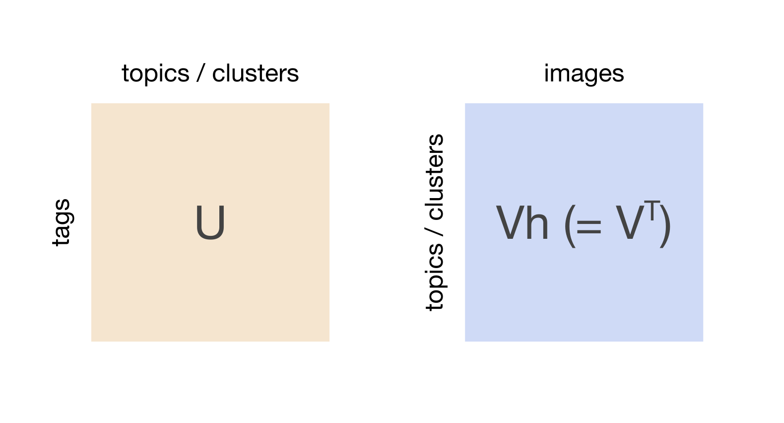
Singular value decomposition (SVD)
%%time
U, s, Vh = scipy.linalg.svd(occurrence_matrix.toarray(), full_matrices=False)
U.shape, s.shape, Vh.shape
CPU times: user 3min 4s, sys: 1.03 s, total: 3min 5s Wall time: 46.9 s
rows = 9
cols = 7
plot = plt.figure(figsize=(16.5, 20))
m = 1
for k in range(1, 1+10*rows, 10):
r = np.array(images)[np.argsort(Vh[k])[:2*cols:2]]
for q in r:
img = imageio.imread(f'/home/dominik/Datasets/Unsplash/datasets/squarecrop-200px/images/{q}.jpg')
plt.subplot(rows, cols, m)
m += 1
plt.imshow(img)
plt.axis('off')
plt.tight_layout(pad=-3.5)
plt.show()
plt.close()
