Sequential Monte Carlo with two gaussians
%matplotlib inline
import pymc3 as pm
import numpy as np
import matplotlib.pyplot as plt

from pymc3.step_methods import smc
import theano.tensor as tt
import shutil

plt.style.use('seaborn-darkgrid')
print('Running on PyMC3 v{}'.format(pm.__version__))
Running on PyMC3 v3.4.1
Sampling from $n$-dimensional distributions with multiple peaks with a standard Metropolis-Hastings algorithm can be difficult, if not impossible, as the Markov chain often gets stuck in either of the minima.
A Sequential Monte Carlo sampler (SMC) is a way to overcome this problem, or at least to ameliorate it. SMC samplers are very similar to genetic algorithms, which are biologically-inspired algorithms that can be summarized as follows:
- Initialization: set a population of individuals
- Mutation: individuals are somehow modified or perturbed
- Selection: individuals with high fitness have higher chance to generate offspring.
- Iterate by using individuals from 3 to set the population in 1.
If each individual is a particular solution to a problem, then a genetic algorithm will eventually produce good solutions to that problem. One key aspect is to generate enough diversity (mutation step) to explore the solution space avoiding getting trap in local minima and then apply selection to probabilistically keep reasonable solutions while also keeping some diversity. Being too greedy and short-sighted could be problematic, bad solutions in a given moment could lead to good solutions in the future.
Moving into the realm of Bayesian statistics each individual is a point in the posterior space, mutations can be done in several ways, a general solution is to use a MCMC method (like Metropolis-Hastings) and run many Markov chains in parallel. The fitness is given by the posterior, points with low posterior density will be removed and points high posterior density will be used as the starting point of a next round of Markov chains (This step is known as reweighting in the SMC literature). The size of the population is kept fixed at some predefined value, so if a point is removed some other point should be used to start at least two new Markov chains.
The previous paragraph is summarized in the next figure, the first subplot show 5 samples (orange dots) at some particular stage. The second subplots show how this samples are reweighted according to the their posterior density (blue Gaussian curve). The third subplot shows the result of running a certain number of Metropolis steps, starting from the selected/reweighting samples in the second subplots, notice how the two samples with the lower posterior density (smaller circles) are discarded and not used to seed Markov chains.
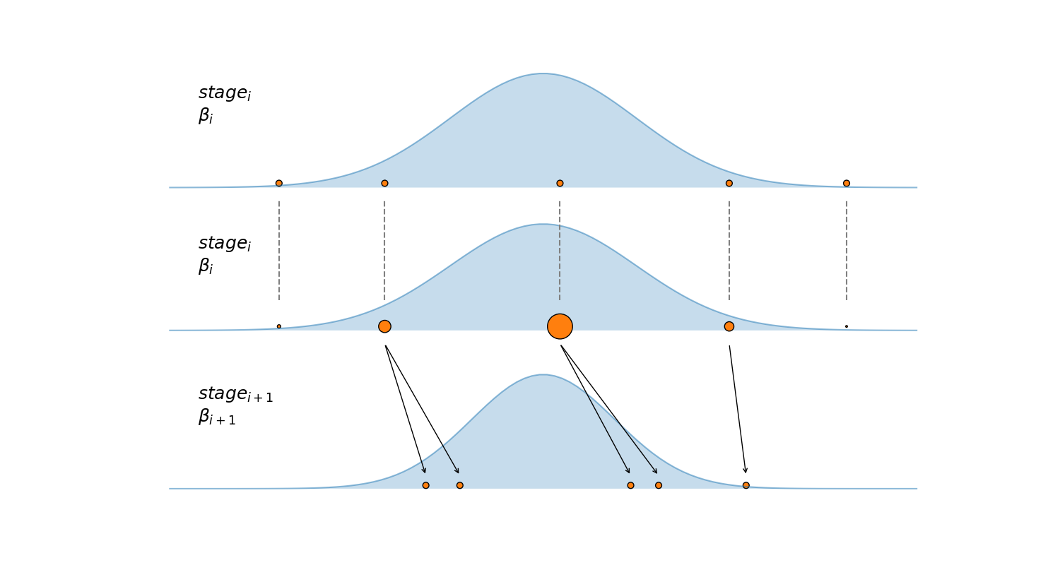
So far we have that the SMC sampler is just a bunch of parallel Markov chains, not very impressive, right? Well not that fast. SMC proceed by moving sequentially trough a series of stages, starting from a simple to sample distribution until it get to the posterior distribution. All this intermediate distribution (or tempered posterior distributions) are controlled by tempering parameter called $\beta$. SMC takes this idea from other tempering methods originated from a branch of physics known as statistical mechanics. The idea is as follow the number of accessible states a real physical system can reach is controlled by the temperature, if the temperature is the lowest possible ($0$ Kelvin) the system is trapped in a single state, on the contrary if the temperature is $\infty$ all states are equally accessible! In the statistical mechanics literature $\beta$ is know as the inverse temperature, the higher the more constrained the system is. Going back to the Bayesian statistics context a natural analogy to these physical systems is given by the following formula:
$$p(\theta \mid y)_{\beta} \propto p(y \mid \theta)^{\beta} p(\theta)$$When $\beta = 0$, the tempered posterior is just the prior and when $\beta=1$ the tempered posterior is the true posterior. SMC starts with $\beta = 0$ and progress by always increasing the value of $\beta$, at each stage, until it reach 1. This is represented in the avobe figure by a narrower Gaussian distribution in the third subplot.
At each stage SMC will use chains independent Markov chains to explore the tempered posterior (the black arrow in the figure). The final samples, i.e those stored in the trace, will be taken exclusively from the final stage ($\beta = 1$), i.e. the true posterior. The final samples are taken from all the chains, thus if you used 100 chains and want 2000 final samples, SMC will use 100 chains, by sampling with replacement, to seed 2000 Markov chains. Those chains will runs for n_steps steps and the end points will be included in the final trace.
The successive values of $\beta$ are determined automatically from the sampling results of the previous intermediate distribution. SMC will try to keep the effective samples size (ESS) constant. Thus, the harder the distribution is to sample the larger the number of stages SMC will take. In other words the cooling will be slow and the successive values of $\beta$ will change in small steps.
Two more parameters that are automatically determined are:
- The number of steps each Markov chain takes to explore the tempered posterior (
n_steps) is determined from the acceptance rate at each stage, SMC use a tune_interval to do this. - The width of the proposal distribution (
MultivariateProposal) is also adjusted adaptively based on the acceptance rate at each stage.
Even when SMC uses the Metropolis-Hasting algorithm under the hood, it has several advantages over it:
- It can sample from $n$-dimensional distributions with multiple peaks.
- It does not have a burn-in period, it starts by sampling directly from the prior and then at each stage the starting points are already distributed according to the tempered posterior (due to the re-weighting step).
- It is inherently parallel.
The number of Markov chains and the number of steps each Markov chain is sampling has to be defined, as well as the tune_interval and the number of processors to be used in the parallel sampling. In this very simple example using only one processor is faster than forking the interpreter. However, if the calculation cost of the model increases it becomes more efficient to use many processors.
chains = 500
Define the number of dimensions for the multivariate gaussians, their weights and the covariance matrix.
n = 4

mu1 = np.ones(n) * (1. / 2)
mu2 = -mu1

stdev = 0.1
sigma = np.power(stdev, 2) * np.eye(n)
isigma = np.linalg.inv(sigma)
dsigma = np.linalg.det(sigma)

w1 = 0.1
w2 = (1 - w1)
The PyMC3 model. Note that we are making two gaussians, where one has w1 (90%) of the mass:
def two_gaussians(x):
    log_like1 = - 0.5 * n * tt.log(2 * np.pi) \
                - 0.5 * tt.log(dsigma) \
                - 0.5 * (x - mu1).T.dot(isigma).dot(x - mu1)
    log_like2 = - 0.5 * n * tt.log(2 * np.pi) \
                - 0.5 * tt.log(dsigma) \
                - 0.5 * (x - mu2).T.dot(isigma).dot(x - mu2)
    return tt.log(w1 * tt.exp(log_like1) + w2 * tt.exp(log_like2))


with pm.Model() as ATMIP_test:
    X = pm.Uniform('X',
                   shape=n,
                   lower=-2. * np.ones_like(mu1),
                   upper=2. * np.ones_like(mu1),
                   testval=-1. * np.ones_like(mu1))
    llk = pm.Potential('llk', two_gaussians(X))
Note: In contrast to other pymc3 samplers here we have to define a random variable like that contains the model likelihood. The likelihood has to be stored in the sampling traces along with the model parameter samples, in order to determine the coefficient of variation [COV] in each transition stage.
Finally, we initialise the sampler and execute the sampling:
with ATMIP_test:
    trace = pm.sample(5000, chains=chains, step=pm.SMC())
Adding model likelihood to RVs!
Init new trace!
Sample initial stage: ...
Beta: 0.000000 Stage: 0
Initializing chain traces ...
Sampling ...
100%|██████████| 500/500 [00:00<00:00, 6000.71it/s]
Beta: 0.009674 Stage: 1
Initializing chain traces ...
Sampling ...
100%|██████████| 500/500 [00:01<00:00, 334.09it/s]
Beta: 0.019848 Stage: 2
Initializing chain traces ...
Sampling ...
100%|██████████| 500/500 [00:00<00:00, 1059.23it/s]
Beta: 0.035439 Stage: 3
Initializing chain traces ...
Sampling ...
100%|██████████| 500/500 [00:00<00:00, 624.93it/s]
Beta: 0.065176 Stage: 4
Initializing chain traces ...
Sampling ...
100%|██████████| 500/500 [00:00<00:00, 736.17it/s]
Beta: 0.132725 Stage: 5
Initializing chain traces ...
Sampling ...
100%|██████████| 500/500 [00:01<00:00, 254.47it/s]
Beta: 0.285900 Stage: 6
Initializing chain traces ...
Sampling ...
100%|██████████| 500/500 [00:01<00:00, 256.10it/s]
Beta: 0.593902 Stage: 7
Initializing chain traces ...
Sampling ...
100%|██████████| 500/500 [00:01<00:00, 253.74it/s]
Beta > 1.: 1.189846
Sample final stage
Initializing chain traces ...
Sampling ...
100%|██████████| 5000/5000 [00:15<00:00, 313.25it/s]
Note: Complex models run for a long time and might stop for some reason during the sampling. In order to restart the sampling in the stage when the sampler stopped, set the stage argument to the right stage number(stage=4). The rm_flag determines whether existing results are deleted - there is NO additional warning, so the user should pay attention to that one!
Plotting the results using the traceplot:
pm.traceplot(trace);
