Using Google BigQuery With Plotly and Pandas
In this IPython Notebook, we will learn about integrating Google's BigQuery with Plotly.
We will query a BigQuery dataset and visualize the results using the Plotly library.
What is BigQuery?
It's a service by Google, which enables analysis of massive datasets. You can use the traditional SQL-like language to query the data.
You can host your own data on BigQuery to use the super fast performance at scale.
Google BigQuery Public Datasets
There are a few datasets stored in BigQuery, available for general public to use.
Some of the publicly available datasets are:
- Hacker News (stories and comments)
- USA Baby Names
- GitHub activity data
- USA disease surveillance
We will use the Hacker News dataset for our analysis.
import pandas as pd

# to communicate with Google BigQuery
from pandas.io import gbq
import plotly.plotly as py
import plotly.graph_objs as go
from plotly.tools import FigureFactory as FF
Prerequisites
You need to have the following libraries:
- python-gflags
- httplib2
- google-api-python-client
Create Project
A project can be created on the Google Developer Console.
Enable BigQuery API
You need to activate the BigQuery API for the project.
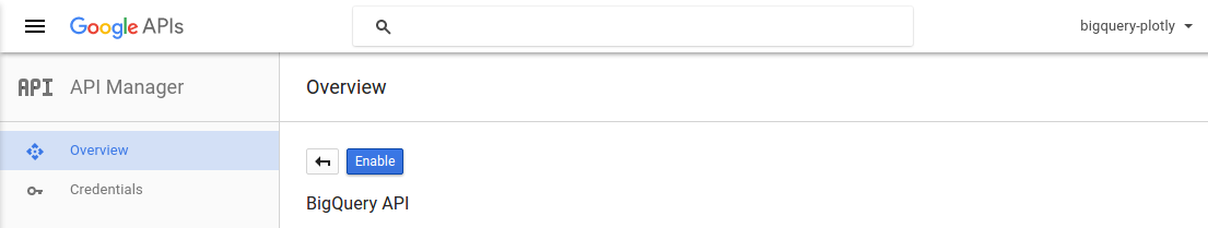
You will have find the Project ID for your project to get the queries working.
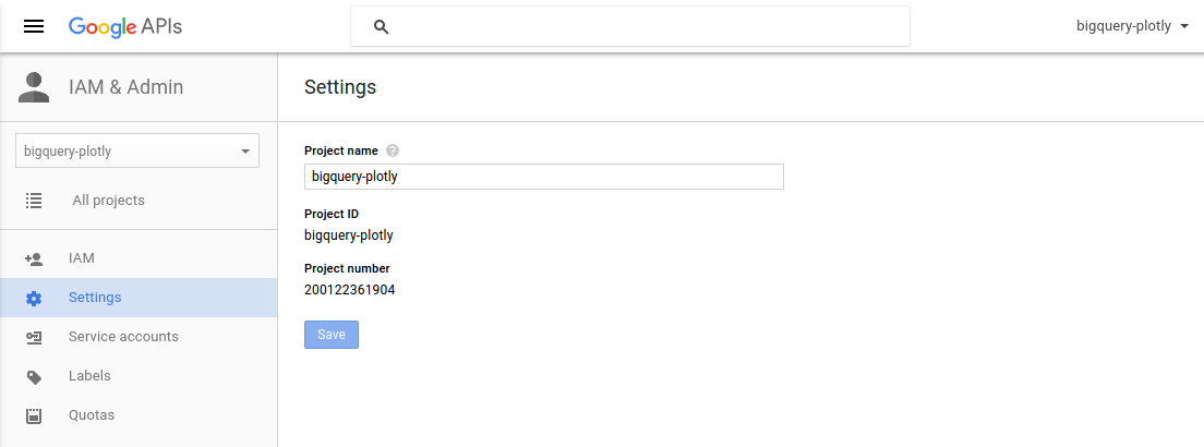
project_id = 'bigquery-plotly'
Top 10 Most Active Users on Hacker News (by total stories submitted)
We will select the top 10 high scoring authors and their respective score values.
top10_active_users_query = """
SELECT
  author AS User,
  count(author) as Stories
FROM
  [fh-bigquery:hackernews.stories]
GROUP BY
  User
ORDER BY
  Stories DESC
LIMIT
  10
"""
The pandas.gbq module provides a method read_gbq to query the BigQuery stored dataset and stores the result as a DataFrame.
try:
    top10_active_users_df = gbq.read_gbq(top10_active_users_query, project_id=project_id)
except:
    print 'Error reading the dataset'
Requesting query... ok.
Query running...
  Elapsed 8.74 s. Waiting...
Query done.
Cache hit.

Retrieving results...
  Got page: 1; 100.0% done. Elapsed 9.36 s.
Got 10 rows.

Total time taken 9.37 s.
Finished at 2016-07-19 17:28:38.
Here is the resultant DataFrame from the query.
top10_active_users_df
| User | Stories | |
|---|---|---|
| 0 | cwan | 7077 |
| 1 | shawndumas | 6602 |
| 2 | evo_9 | 5659 |
| 3 | nickb | 4322 |
| 4 | iProject | 4266 |
| 5 | bootload | 4212 |
| 6 | edw519 | 3844 |
| 7 | ColinWright | 3766 |
| 8 | nreece | 3724 |
| 9 | tokenadult | 3659 |
Using the create_table method from the FigureFactory module, we can generate a table from the resulting DataFrame.
top_10_users_table = FF.create_table(top10_active_users_df)
py.iplot(top_10_users_table, filename='top-10-active-users')
Top 10 Hacker News Submissions (by score)
We will select the title and score columns in the descending order of their score, keeping only top 10 stories among all.
top10_story_query = """
SELECT
  title,
  score,
  time_ts AS timestamp
FROM
  [fh-bigquery:hackernews.stories]
ORDER BY
  score DESC
LIMIT
  10
"""
try:
    top10_story_df = gbq.read_gbq(top10_story_query, project_id=project_id)
except:
    print 'Error reading the dataset'
Requesting query... ok.
Query running...
  Elapsed 13.54 s. Waiting...
Query done.
Cache hit.

Retrieving results...
  Got page: 1; 100.0% done. Elapsed 14.34 s.
Got 10 rows.

Total time taken 14.34 s.
Finished at 2016-07-19 17:28:57.
# Create a table figure from the DataFrame
top10_story_figure = FF.create_table(top10_story_df)

# Scatter trace for the bubble chart timeseries
story_timeseries_trace = go.Scatter(
    x=top10_story_df['timestamp'],
    y=top10_story_df['score'],
    xaxis='x2',
    yaxis='y2',
    mode='markers',
    text=top10_story_df['title'],
    marker=dict(
        color=[80 + i*5 for i in range(10)],
        size=top10_story_df['score']/50,
        showscale=False
    )
)

# Add the trace data to the figure
top10_story_figure['data'].extend(go.Data([story_timeseries_trace]))

# Subplot layout
top10_story_figure.layout.yaxis.update({'domain': [0, .45]})
top10_story_figure.layout.yaxis2.update({'domain': [.6, 1]})

# Y-axis of the graph should be anchored with X-axis
top10_story_figure.layout.yaxis2.update({'anchor': 'x2'})
top10_story_figure.layout.xaxis2.update({'anchor': 'y2'})

# Add the height and title attribute
top10_story_figure.layout.update({'height':900})
top10_story_figure.layout.update({'title': 'Highest Scoring Submissions on Hacker News'})

# Update the background color for plot and paper
top10_story_figure.layout.update({'paper_bgcolor': 'rgb(243, 243, 243)'})
top10_story_figure.layout.update({'plot_bgcolor': 'rgb(243, 243, 243)'})

# Add the margin to make subplot titles visible
top10_story_figure.layout.margin.update({'t':75, 'l':50})
top10_story_figure.layout.yaxis2.update({'title': 'Upvote Score'})
top10_story_figure.layout.xaxis2.update({'title': 'Post Time'})
py.image.save_as(top10_story_figure, filename='top10-posts.png')
py.iplot(top10_story_figure, filename='highest-scoring-submissions')
You can see that the lists consist of the stories involving some big names.
- "Death of Steve Jobs and Aaron Swartz"
- "Announcements of the Hyperloop and the game 2048".
- "Microsoft open sourcing the .NET"
The story title is visible when you hover over the bubbles.
tld_share_query = """
SELECT
  TLD(url) AS domain,
  count(score) AS stories
FROM
  [fh-bigquery:hackernews.stories]
GROUP BY
  domain
ORDER BY
  stories DESC
LIMIT 10
"""
try:
    tld_share_df = gbq.read_gbq(tld_share_query, project_id=project_id)
except:
    print 'Error reading the dataset'
Requesting query... ok.
Query running...
Query done.
Cache hit.

Retrieving results...
  Got page: 1; 100.0% done. Elapsed 7.09 s.
Got 10 rows.

Total time taken 7.09 s.
Finished at 2016-07-19 17:29:10.
tld_share_df
| domain | stories | |
|---|---|---|
| 0 | .com | 1324329 |
| 1 | .org | 120716 |
| 2 | None | 111744 |
| 3 | .net | 58754 |
| 4 | .co.uk | 43955 |
| 5 | .io | 23507 |
| 6 | .edu | 14727 |
| 7 | .co | 10692 |
| 8 | .me | 10565 |
| 9 | .info | 8121 |
labels = tld_share_df['domain']
values = tld_share_df['stories']

tld_share_trace = go.Pie(labels=labels, values=values)
data = [tld_share_trace]

layout = go.Layout(
    title='Submissions shared by Top-level domains'
)

fig = go.Figure(data=data, layout=layout)
py.iplot(fig)
We can notice that the .com top-level domain contributes to most of the stories on Hacker News.
Public response to the "Who Is Hiring?" posts
There is an account on Hacker News by the name whoishiring.
This account automatically submits a 'Who is Hiring?' post at 11 AM Eastern time on the first weekday of every month.
wih_query = """
SELECT
  id,
  title,
  score,
  time_ts
FROM
  [fh-bigquery:hackernews.stories]
WHERE
  author == 'whoishiring' AND
  LOWER(title) contains 'who is hiring?'
ORDER BY
  time
"""
try:
    wih_df = gbq.read_gbq(wih_query, project_id=project_id)
except:
    print 'Error reading the dataset'
Requesting query... ok.
Query running...
Query done.
Cache hit.

Retrieving results...
Got 52 rows.

Total time taken 4.73 s.
Finished at 2016-07-19 17:29:19.
trace = go.Scatter(
    x=wih_df['time_ts'],
    y=wih_df['score'],
    mode='markers+lines',
    text=wih_df['title'],
    marker=dict(
        size=wih_df['score']/50
    )
)

layout = go.Layout(
    title='Public response to the "Who Is Hiring?" posts',
    xaxis=dict(
        title="Post Time"
    ),
    yaxis=dict(
        title="Upvote Score"
    )
)

data = [trace]

fig = go.Figure(data=data, layout=layout)
py.iplot(fig, filename='whoishiring-public-response')
Submission Traffic Volume in a Week
week_traffic_query = """
SELECT
  DAYOFWEEK(time_ts) as Weekday,
  count(DAYOFWEEK(time_ts)) as story_counts
FROM
  [fh-bigquery:hackernews.stories]
GROUP BY
  Weekday
ORDER BY
  Weekday
"""
try:
    week_traffic_df = gbq.read_gbq(week_traffic_query, project_id=project_id)
except:
    print 'Error reading the dataset'
Requesting query... ok.
Query running...
Query done.
Cache hit.

Retrieving results...
Got 8 rows.

Total time taken 5.26 s.
Finished at 2016-07-19 17:29:29.
week_traffic_df['Day'] = ['NULL', 'Sunday', 'Monday', 'Tuesday', 'Wednesday', 'Thursday', 'Friday', 'Saturday']
week_traffic_df = week_traffic_df.drop(week_traffic_df.index[0])
trace = go.Scatter(
    x=week_traffic_df['Day'],
    y=week_traffic_df['story_counts'],
    mode='lines',
    text=week_traffic_df['Day']
)

layout = go.Layout(
    title='Submission Traffic Volume (Week Days)',
    xaxis=dict(
        title="Day of the Week"
    ),
    yaxis=dict(
        title="Total Submissions"
    )
)

data = [trace]

fig = go.Figure(data=data, layout=layout)
py.iplot(fig, filename='submission-traffic-volume')
We can observe that the Hacker News faces fewer submissions during the weekends.
Programming Language Trend on HackerNews
We will compare the trends for the Python and PHP programming languages, using the Hacker News post titles.
python_query = """
SELECT
  YEAR(time_ts) as years,
  COUNT(YEAR(time_ts )) as trends
FROM
  [fh-bigquery:hackernews.stories]
WHERE
  LOWER(title) contains 'python'
GROUP BY
  years
ORDER BY
  years
"""

php_query = """
SELECT
  YEAR(time_ts) as years,
  COUNT(YEAR(time_ts )) as trends
FROM
  [fh-bigquery:hackernews.stories]
WHERE
  LOWER(title) contains 'php'
GROUP BY
  years
ORDER BY
  years
"""
try:
    python_df = gbq.read_gbq(python_query, project_id=project_id)
except:
    print 'Error reading the dataset'
Requesting query... ok.
Query running...
  Elapsed 10.07 s. Waiting...
Query done.
Cache hit.

Retrieving results...
  Got page: 1; 100.0% done. Elapsed 10.92 s.
Got 9 rows.

Total time taken 10.93 s.
Finished at 2016-07-19 17:29:44.
try:
    php_df = gbq.read_gbq(php_query, project_id=project_id)
except:
    print 'Error reading the dataset'
Requesting query... ok.
Query running...
  Elapsed 9.28 s. Waiting...
Query done.
Cache hit.

Retrieving results...
  Got page: 1; 100.0% done. Elapsed 9.91 s.
Got 9 rows.

Total time taken 9.92 s.
Finished at 2016-07-19 17:29:54.
trace1 = go.Scatter(
    x=python_df['years'],
    y=python_df['trends'],
    mode='lines',
    line=dict(color='rgba(115,115,115,1)', width=4),
    connectgaps=True,
)

trace2 = go.Scatter(
    x=[python_df['years'][0], python_df['years'][8]],
    y=[python_df['trends'][0], python_df['trends'][8]],
    mode='markers',
    marker=dict(color='rgba(115,115,115,1)', size=8)
)

trace3 = go.Scatter(
    x=php_df['years'],
    y=php_df['trends'],
    mode='lines',
    line=dict(color='rgba(189,189,189,1)', width=4),
    connectgaps=True,
)

trace4 = go.Scatter(
    x=[php_df['years'][0], php_df['years'][8]],
    y=[php_df['trends'][0], php_df['trends'][8]],
    mode='markers',
    marker=dict(color='rgba(189,189,189,1)', size=8)
)

traces = [trace1, trace2, trace3, trace4]

layout = go.Layout(
    xaxis=dict(
        showline=True,
        showgrid=False,
        showticklabels=True,
        linecolor='rgb(204, 204, 204)',
        linewidth=2,
        autotick=False,
        ticks='outside',
        tickcolor='rgb(204, 204, 204)',
        tickwidth=2,
        ticklen=5,
        tickfont=dict(
            family='Arial',
            size=12,
            color='rgb(82, 82, 82)',
        ),
    ),
    yaxis=dict(
        showgrid=False,
        zeroline=False,
        showline=False,
        showticklabels=False,
    ),
    autosize=False,
    margin=dict(
        autoexpand=False,
        l=100,
        r=20,
        t=110,
    ),
    showlegend=False,
)

annotations = []

annotations.append(
    dict(xref='paper', x=0.95, y=python_df['trends'][8],
    xanchor='left', yanchor='middle',
    text='Python',
    font=dict(
        family='Arial',
        size=14,
        color='rgba(49,130,189, 1)'
    ),
    showarrow=False)
)

annotations.append(
    dict(xref='paper', x=0.95, y=php_df['trends'][8],
    xanchor='left', yanchor='middle',
    text='PHP',
    font=dict(
        family='Arial',
        size=14,
        color='rgba(49,130,189, 1)'
    ),
    showarrow=False)
)

annotations.append(
    dict(xref='paper', yref='paper', x=0.5, y=-0.1,
    xanchor='center', yanchor='top',
    text='Source: Hacker News submissions with the title containing Python/PHP',
    font=dict(
        family='Arial',
        size=12,
        color='rgb(150,150,150)'
    ),
    showarrow=False)
)

layout['annotations'] = annotations

fig = go.Figure(data=traces, layout=layout)
py.iplot(fig, filename='programming-language-trends')
As we already know about this trend, Python is dominating PHP throughout the timespan.