(updated version) Classification product based on a Deep Learning model (by fastai v2)
Use case: Dog & Cat Breeds Recognizer for Veterinary Clinics
- Author: Pierre Guillou (AI Professor at the University of Brasilia (UnB) & AI Lab Associate Researcher in NLP)
- Creation date: 10/22/2020
- Update date: 04/19/2021 (see the 10/22/2020 version)
- Post in Medium: Product based on a Deep Learning model (by fastai v2)
- Github folder of the Web App v1
- Version 1 of the Web App
Overview
This is the notebook of the post Product based on a Deep Learning model (by fastai v2).
Read this post to understand the context and objective of this notebook.
Results
In the notebook 05_pet_breeds.ipynb, the best accuray model is 94.52% (1 - the error rate which is 0.054804).
By using all the fastai techniques tought by Jeremy Howard in the fastai 2020 course, we got an accuracy of 95.81%.
1. Initialization
# Import fastai v2 for computer vision
from fastai.vision.all import *
from fastai.vision.widgets import *
# Check for CUDA & GPU
if torch.cuda.is_available():
    print(f'gpu: {torch.cuda.current_device()} ({torch.cuda.get_device_name()})')
gpu: 0 (Tesla V100-PCIE-32GB)
2. Data
Get path to data
path = untar_data(URLs.PETS)
path.ls()
(#2) [Path('/mnt/home/pierre/.fastai/data/oxford-iiit-pet/annotations'),Path('/mnt/home/pierre/.fastai/data/oxford-iiit-pet/images')]
Display an image
2 ways to display an image from its path in a jupyter notebook.
PILImage.create()
# Check first image
path_to_img = (path/'images').ls()[0]
img = PILImage.create(path_to_img)
img.to_thumb(192)

Image.open()
img = Image.open(path_to_img)
img.to_thumb(192)
Tensor of an image
An image is a matrix of pixels with 2 (black and white) or more channels (3 for RGB). Each pixel has a number from 0 to 255.
# from image to tensor
tensor(img).shape
torch.Size([500, 487, 3])
#hide_output
img_t = tensor(img)
df = pd.DataFrame(img_t[4:15,4:22,0])
# df.style.set_properties(**{'font-size':'6pt'}).background_gradient('Greys')
df.style.set_properties(**{'font-size':'6pt'}).background_gradient()
| 0 | 1 | 2 | 3 | 4 | 5 | 6 | 7 | 8 | 9 | 10 | 11 | 12 | 13 | 14 | 15 | 16 | 17 | |
|---|---|---|---|---|---|---|---|---|---|---|---|---|---|---|---|---|---|---|
| 0 | 202 | 250 | 239 | 169 | 179 | 209 | 235 | 238 | 174 | 236 | 239 | 237 | 245 | 247 | 251 | 243 | 238 | 238 |
| 1 | 114 | 143 | 175 | 158 | 182 | 177 | 143 | 209 | 103 | 232 | 142 | 252 | 253 | 250 | 246 | 248 | 254 | 252 |
| 2 | 111 | 89 | 94 | 101 | 147 | 172 | 136 | 203 | 129 | 222 | 194 | 247 | 240 | 248 | 247 | 243 | 245 | 239 |
| 3 | 94 | 100 | 95 | 84 | 85 | 127 | 198 | 248 | 237 | 220 | 235 | 221 | 219 | 245 | 254 | 246 | 252 | 249 |
| 4 | 99 | 87 | 104 | 112 | 121 | 96 | 102 | 150 | 181 | 199 | 225 | 246 | 237 | 255 | 247 | 234 | 240 | 249 |
| 5 | 87 | 91 | 109 | 128 | 110 | 114 | 91 | 92 | 100 | 144 | 186 | 230 | 219 | 219 | 231 | 239 | 241 | 247 |
| 6 | 96 | 91 | 91 | 171 | 140 | 90 | 97 | 95 | 102 | 92 | 114 | 149 | 187 | 225 | 239 | 247 | 243 | 251 |
| 7 | 96 | 96 | 95 | 104 | 126 | 94 | 94 | 92 | 90 | 91 | 84 | 105 | 112 | 164 | 233 | 238 | 239 | 246 |
| 8 | 112 | 104 | 101 | 88 | 81 | 102 | 97 | 92 | 94 | 102 | 103 | 103 | 112 | 100 | 133 | 196 | 231 | 240 |
| 9 | 110 | 97 | 91 | 97 | 93 | 98 | 89 | 98 | 98 | 110 | 120 | 116 | 125 | 110 | 113 | 106 | 137 | 173 |
| 10 | 114 | 108 | 99 | 95 | 98 | 103 | 100 | 88 | 100 | 109 | 104 | 94 | 103 | 101 | 109 | 118 | 108 | 103 |
# from tensor to image
show_image(img_t);

3. Dataloaders
We will define a DataBlock() object using all the recent techniques (see the notebook 07_sizing_and_tta.ipynb):
- Presizing (notebook 05_pet_breeds.ipynb).
- Data Augmentation with the list of transforms at batch level (
aug_transforms()). - Normalization with the standard ImageNet mean and standard deviation (
Normalize.from_stats(*imagenet_stats)). - Progressive Resizing: Gradually using larger and larger images as you train (
get_dls()).
# Progressive Resizing
def get_dls(bs, size):
    dblock = DataBlock(blocks = (ImageBlock, CategoryBlock),
                       get_items=get_image_files,
                       splitter=RandomSplitter(seed=42),
                       get_y=using_attr(RegexLabeller(r'(.+)_\d+.jpg$'), 'name'),
                       item_tfms=RandomResizedCrop(460, min_scale=0.3),           # presizing
                       batch_tfms=[*aug_transforms(size=size, min_scale=0.75),    # data augmentation
                                   Normalize.from_stats(*imagenet_stats)])        # normalization
    return dblock.dataloaders(path/"images", bs=bs)
Note: The *args and **kwargs is a common idiom to allow arbitrary number of arguments to functions as described in the section more on defining functions in the Python documentation (source).
# Get Dataloaders
dls = get_dls(128, 128)
# Check number of categories and list
dls.vocab
['Abyssinian', 'Bengal', 'Birman', 'Bombay', 'British_Shorthair', 'Egyptian_Mau', 'Maine_Coon', 'Persian', 'Ragdoll', 'Russian_Blue', 'Siamese', 'Sphynx', 'american_bulldog', 'american_pit_bull_terrier', 'basset_hound', 'beagle', 'boxer', 'chihuahua', 'english_cocker_spaniel', 'english_setter', 'german_shorthaired', 'great_pyrenees', 'havanese', 'japanese_chin', 'keeshond', 'leonberger', 'miniature_pinscher', 'newfoundland', 'pomeranian', 'pug', 'saint_bernard', 'samoyed', 'scottish_terrier', 'shiba_inu', 'staffordshire_bull_terrier', 'wheaten_terrier', 'yorkshire_terrier']
# Batch size and Check images in training batch
dls.bs, dls.show_batch(nrows=1, ncols=3)
(128, None)

# Batch size and Check images in training batch
dls.bs, dls.train.show_batch(nrows=1, ncols=5, unique=True)
(128, None)

# Batch size and Check images in training batch
dls.bs, dls.valid.show_batch(nrows=1, ncols=5, unique=True)
(128, None)

4. First model (baseline)
To encourage our model to be less confident, we'll use label smoothing that will make our training more robust, even if there is mislabeled data. The result will be a model that generalizes better (see the notebook 07_sizing_and_tta.ipynb).
Let's train our model with the following fine-tuning techniques:
- Label smoothing in order to avoid that our model is too confident.
- Weighted loss in order to take into account the training dataset distribution (key point when it is unbalanced)
- Gradual unfreezing of layers from the last ones to the first ones.
- Discriminative Learning Rates (notebook 05_pet_breeds.ipynb).
- Deeper Architectures: let's start with resnet34 as baseline, and then resnet152 as final model.
To get the validation accuracy, we will use Test Time Augmentation (TTA).
4.1 Images of size 128
# Learner with model resnet34
dls = get_dls(128, 128)
model = resnet34

learn = cnn_learner(dls, model, metrics=[accuracy])
Weighted loss
Get the training distribution by category and visualize it.
from collections import Counter

# number of items by category
labels_list = [dls.train_ds[i][1].item() for i in range(len(dls.train_ds))]
count_dict = dict(Counter(labels_list).items())
plt.bar(count_dict.keys(), count_dict.values())
plt.show()

Our training dataset is balanced but let's change the loss to a weighted loss in order to show how to do it.
trn_LabelCounts = np.array([count_dict[i] for i in range(dls.c)])
trn_weights = [1 - count/(len(dls.train_ds)) for count in trn_LabelCounts]
# original loss function
learn.loss_func
FlattenedLoss of CrossEntropyLoss()
# change the loss function
loss_weights = torch.FloatTensor(trn_weights).cuda()
learn.loss_func = LabelSmoothingCrossEntropyFlat(weight=loss_weights)

# weighted loss function
learn.loss_func
FlattenedLoss of LabelSmoothingCrossEntropy()
Freeze all layers but the last (new) ones
# Check model and frozen layers
learn.freeze()
learn.summary()
Sequential (Input shape: 128)
============================================================================
Layer (type)         Output Shape         Param #    Trainable
============================================================================
                     128 x 64 x 64 x 64
Conv2d                                    9408       False
BatchNorm2d                               128        True
ReLU
MaxPool2d
Conv2d                                    36864      False
BatchNorm2d                               128        True
ReLU
Conv2d                                    36864      False
BatchNorm2d                               128        True
Conv2d                                    36864      False
BatchNorm2d                               128        True
ReLU
Conv2d                                    36864      False
BatchNorm2d                               128        True
Conv2d                                    36864      False
BatchNorm2d                               128        True
ReLU
Conv2d                                    36864      False
BatchNorm2d                               128        True
____________________________________________________________________________
                     128 x 128 x 16 x 16
Conv2d                                    73728      False
BatchNorm2d                               256        True
ReLU
Conv2d                                    147456     False
BatchNorm2d                               256        True
Conv2d                                    8192       False
BatchNorm2d                               256        True
Conv2d                                    147456     False
BatchNorm2d                               256        True
ReLU
Conv2d                                    147456     False
BatchNorm2d                               256        True
Conv2d                                    147456     False
BatchNorm2d                               256        True
ReLU
Conv2d                                    147456     False
BatchNorm2d                               256        True
Conv2d                                    147456     False
BatchNorm2d                               256        True
ReLU
Conv2d                                    147456     False
BatchNorm2d                               256        True
____________________________________________________________________________
                     128 x 256 x 8 x 8
Conv2d                                    294912     False
BatchNorm2d                               512        True
ReLU
Conv2d                                    589824     False
BatchNorm2d                               512        True
Conv2d                                    32768      False
BatchNorm2d                               512        True
Conv2d                                    589824     False
BatchNorm2d                               512        True
ReLU
Conv2d                                    589824     False
BatchNorm2d                               512        True
Conv2d                                    589824     False
BatchNorm2d                               512        True
ReLU
Conv2d                                    589824     False
BatchNorm2d                               512        True
Conv2d                                    589824     False
BatchNorm2d                               512        True
ReLU
Conv2d                                    589824     False
BatchNorm2d                               512        True
Conv2d                                    589824     False
BatchNorm2d                               512        True
ReLU
Conv2d                                    589824     False
BatchNorm2d                               512        True
Conv2d                                    589824     False
BatchNorm2d                               512        True
ReLU
Conv2d                                    589824     False
BatchNorm2d                               512        True
____________________________________________________________________________
                     128 x 512 x 4 x 4
Conv2d                                    1179648    False
BatchNorm2d                               1024       True
ReLU
Conv2d                                    2359296    False
BatchNorm2d                               1024       True
Conv2d                                    131072     False
BatchNorm2d                               1024       True
Conv2d                                    2359296    False
BatchNorm2d                               1024       True
ReLU
Conv2d                                    2359296    False
BatchNorm2d                               1024       True
Conv2d                                    2359296    False
BatchNorm2d                               1024       True
ReLU
Conv2d                                    2359296    False
BatchNorm2d                               1024       True
____________________________________________________________________________
                     []
AdaptiveAvgPool2d
AdaptiveMaxPool2d
Flatten
BatchNorm1d                               2048       True
Dropout
____________________________________________________________________________
                     128 x 512
Linear                                    524288     True
ReLU
BatchNorm1d                               1024       True
Dropout
____________________________________________________________________________
                     128 x 37
Linear                                    18944      True
____________________________________________________________________________

Total params: 21,830,976
Total trainable params: 563,328
Total non-trainable params: 21,267,648

Optimizer used: <function Adam at 0x7f9d73a2e3a0>
Loss function: FlattenedLoss of LabelSmoothingCrossEntropy()

Model frozen up to parameter group #2

Callbacks:
  - TrainEvalCallback
  - Recorder
  - ProgressCallback
We can notice that our model is frozen up to parameters group 2 but our model has how many parameters group?
print(f'number of parameters groups: {len(learn.opt.param_groups)}')
number of parameters groups: 3
For more information about parameters group, check "How to create groups of layers and each one with a different Learning Rate?".
# Learning rate
learn.lr_find()
SuggestedLRs(lr_min=0.010000000149011612, lr_steep=0.00363078061491251)

As only the last layers are unfrozen, let's choose the learning rate 10 times less than the one of the loss minimum as lr_max (1e-2).
# Train the model with lr_max and the fit_one_cycle() function on 1 epoch
lr_max = 1e-2
learn.fit_one_cycle(1, lr_max=lr_max)
| epoch | train_loss | valid_loss | accuracy | time |
|---|---|---|---|---|
| 0 | 2.320444 | 1.610688 | 0.746279 | 00:10 |
# Save the model
learn.save('petbreeds_1')
Path('models/petbreeds_1.pth')
# Display the Learning rate and momentum values used in training
learn.recorder.plot_sched()

Unfreeze all layers and Discriminative Learning Rates
# Load model, unfreeze layers and check it
learn = learn.load('petbreeds_1')
learn.unfreeze()
learn.summary()
Sequential (Input shape: 128)
============================================================================
Layer (type)         Output Shape         Param #    Trainable
============================================================================
                     128 x 64 x 64 x 64
Conv2d                                    9408       True
BatchNorm2d                               128        True
ReLU
MaxPool2d
Conv2d                                    36864      True
BatchNorm2d                               128        True
ReLU
Conv2d                                    36864      True
BatchNorm2d                               128        True
Conv2d                                    36864      True
BatchNorm2d                               128        True
ReLU
Conv2d                                    36864      True
BatchNorm2d                               128        True
Conv2d                                    36864      True
BatchNorm2d                               128        True
ReLU
Conv2d                                    36864      True
BatchNorm2d                               128        True
____________________________________________________________________________
                     128 x 128 x 16 x 16
Conv2d                                    73728      True
BatchNorm2d                               256        True
ReLU
Conv2d                                    147456     True
BatchNorm2d                               256        True
Conv2d                                    8192       True
BatchNorm2d                               256        True
Conv2d                                    147456     True
BatchNorm2d                               256        True
ReLU
Conv2d                                    147456     True
BatchNorm2d                               256        True
Conv2d                                    147456     True
BatchNorm2d                               256        True
ReLU
Conv2d                                    147456     True
BatchNorm2d                               256        True
Conv2d                                    147456     True
BatchNorm2d                               256        True
ReLU
Conv2d                                    147456     True
BatchNorm2d                               256        True
____________________________________________________________________________
                     128 x 256 x 8 x 8
Conv2d                                    294912     True
BatchNorm2d                               512        True
ReLU
Conv2d                                    589824     True
BatchNorm2d                               512        True
Conv2d                                    32768      True
BatchNorm2d                               512        True
Conv2d                                    589824     True
BatchNorm2d                               512        True
ReLU
Conv2d                                    589824     True
BatchNorm2d                               512        True
Conv2d                                    589824     True
BatchNorm2d                               512        True
ReLU
Conv2d                                    589824     True
BatchNorm2d                               512        True
Conv2d                                    589824     True
BatchNorm2d                               512        True
ReLU
Conv2d                                    589824     True
BatchNorm2d                               512        True
Conv2d                                    589824     True
BatchNorm2d                               512        True
ReLU
Conv2d                                    589824     True
BatchNorm2d                               512        True
Conv2d                                    589824     True
BatchNorm2d                               512        True
ReLU
Conv2d                                    589824     True
BatchNorm2d                               512        True
____________________________________________________________________________
                     128 x 512 x 4 x 4
Conv2d                                    1179648    True
BatchNorm2d                               1024       True
ReLU
Conv2d                                    2359296    True
BatchNorm2d                               1024       True
Conv2d                                    131072     True
BatchNorm2d                               1024       True
Conv2d                                    2359296    True
BatchNorm2d                               1024       True
ReLU
Conv2d                                    2359296    True
BatchNorm2d                               1024       True
Conv2d                                    2359296    True
BatchNorm2d                               1024       True
ReLU
Conv2d                                    2359296    True
BatchNorm2d                               1024       True
____________________________________________________________________________
                     []
AdaptiveAvgPool2d
AdaptiveMaxPool2d
Flatten
BatchNorm1d                               2048       True
Dropout
____________________________________________________________________________
                     128 x 512
Linear                                    524288     True
ReLU
BatchNorm1d                               1024       True
Dropout
____________________________________________________________________________
                     128 x 37
Linear                                    18944      True
____________________________________________________________________________

Total params: 21,830,976
Total trainable params: 21,830,976
Total non-trainable params: 0

Optimizer used: <function Adam at 0x7f9d73a2e3a0>
Loss function: FlattenedLoss of LabelSmoothingCrossEntropy()

Model unfrozen

Callbacks:
  - TrainEvalCallback
  - Recorder
  - ProgressCallback
Note: we can verify with learn.summary() that all parameters are unfrozen.
# Learning rate
learn.lr_find()
SuggestedLRs(lr_min=6.918309954926372e-05, lr_steep=4.786300905834651e-06)

As we unfroze all layers of the model, let's choose the learning rate of the loss minimum as lr_max (1e-3) and use the Discriminative Learning Rates technique.
# Train the model with lr_max and the fit_one_cycle() function on 1 epoch
lr_max = 1e-3
lr_min = lr_max / 100
learn.fit_one_cycle(10, lr_max=slice(lr_min,lr_max))
| epoch | train_loss | valid_loss | accuracy | time |
|---|---|---|---|---|
| 0 | 1.718739 | 1.433060 | 0.799053 | 00:11 |
| 1 | 1.599868 | 1.333921 | 0.820027 | 00:11 |
| 2 | 1.490716 | 1.292866 | 0.813938 | 00:11 |
| 3 | 1.400105 | 1.210695 | 0.844384 | 00:11 |
| 4 | 1.306173 | 1.173454 | 0.857916 | 00:11 |
| 5 | 1.222220 | 1.134675 | 0.867388 | 00:11 |
| 6 | 1.151358 | 1.127675 | 0.864682 | 00:10 |
| 7 | 1.110902 | 1.088684 | 0.878214 | 00:11 |
| 8 | 1.087477 | 1.090277 | 0.879567 | 00:11 |
| 9 | 1.074081 | 1.089503 | 0.876184 | 00:11 |
# Save the model
learn.save('petbreeds_2')
Path('models/petbreeds_2.pth')
# all recorded values
learn.recorder.values
[(#3) [1.7187391519546509,1.4330599308013916,0.7990527749061584],
 (#3) [1.5998684167861938,1.3339207172393799,0.8200270533561707],
 (#3) [1.4907162189483643,1.2928661108016968,0.813937783241272],
 (#3) [1.4001049995422363,1.210694670677185,0.8443843126296997],
 (#3) [1.3061734437942505,1.1734542846679688,0.8579161167144775],
 (#3) [1.2222195863723755,1.13467538356781,0.8673883676528931],
 (#3) [1.1513580083847046,1.12767493724823,0.8646820187568665],
 (#3) [1.1109017133712769,1.0886842012405396,0.8782138228416443],
 (#3) [1.0874768495559692,1.0902774333953857,0.8795669674873352],
 (#3) [1.0740807056427002,1.0895026922225952,0.8761840462684631]]
# Display the training and validation loss
learn.recorder.plot_loss()

# Validation accuracy
plt.plot(L(learn.recorder.values).itemgot(2));

# Train loss, Valid loss and accuracy of the model
learn.recorder.values[-1]
(#3) [1.0740807056427002,1.0895026922225952,0.8761840462684631]
# Valid accuracy of the model
print(round(learn.recorder.values[-1][-1]*100,2),'%')
87.62 %
We can visualize the model results on the validation set, too.
learn.show_results(ds_idx=1, nrows=3, figsize=(16,8))

4.2 Images of size 224
# Learner with model resnet34
dls = get_dls(64, 224)
model = resnet34
loss_func = LabelSmoothingCrossEntropyFlat(weight=loss_weights)

learn = cnn_learner(dls, model, loss_func=loss_func, metrics=[accuracy])
learn = learn.load('petbreeds_2')
Freeze all layers but the last (new) ones
# Learning rate
learn.freeze()
learn.lr_find()
SuggestedLRs(lr_min=0.0006309573538601399, lr_steep=1.2022644114040304e-05)

As only the last layers are unfrozen, let's choose the learning rate 10 times less than the one of the loss minimum as lr_max (1e-3).
# Train the model with lr_max and the fit_one_cycle() function on 1 epoch
lr_max = 1e-3
learn.fit_one_cycle(1, lr_max=lr_max)
| epoch | train_loss | valid_loss | accuracy | time |
|---|---|---|---|---|
| 0 | 1.099601 | 0.950549 | 0.935047 | 00:15 |
# Save the model
learn.save('petbreeds_3')
Path('models/petbreeds_3.pth')
Unfreeze all layers and Discriminative Learning Rates
# Load model, unfreeze layers and check it
learn = learn.load('petbreeds_3')
learn.unfreeze()
# Learning rate
learn.lr_find()
SuggestedLRs(lr_min=1.9054607491852948e-07, lr_steep=9.12010818865383e-07)

As we unfroze all layers of the model, let's choose the learning rate of the loss minimum as lr_max (1e-4).
# Train the model with lr_max and the fit_one_cycle() function on 1 epoch
lr_max = 1e-4
lr_min = lr_max / 100
learn.fit_one_cycle(10, lr_max=slice(lr_min,lr_max))
| epoch | train_loss | valid_loss | accuracy | time |
|---|---|---|---|---|
| 0 | 1.057191 | 0.946043 | 0.939107 | 00:18 |
| 1 | 1.047280 | 0.941114 | 0.935724 | 00:18 |
| 2 | 1.032457 | 0.931538 | 0.935724 | 00:18 |
| 3 | 1.024848 | 0.925354 | 0.938430 | 00:17 |
| 4 | 1.013020 | 0.923876 | 0.939107 | 00:17 |
| 5 | 0.998921 | 0.914864 | 0.938430 | 00:18 |
| 6 | 0.996773 | 0.917239 | 0.941137 | 00:18 |
| 7 | 0.998383 | 0.910425 | 0.945873 | 00:17 |
| 8 | 0.987399 | 0.909182 | 0.942490 | 00:17 |
| 9 | 0.980322 | 0.910274 | 0.943843 | 00:17 |
# Save the model
learn.save('petbreeds_4')
Path('models/petbreeds_4.pth')
# Display the training and validation loss
learn.recorder.plot_loss()

# Validation accuracy
plt.plot(L(learn.recorder.values).itemgot(2));

# Valid accuracy of the model
print(round(learn.recorder.values[-1][-1]*100,2),'%')
94.38 %
# Test Time Augmentation
# notebook: https://github.com/fastai/fastbook/blob/master/07_sizing_and_tta.ipynb
learn.epoch = 0
preds,targs = learn.tta()
accuracy(preds, targs).item()
0.9519621133804321
Let's keep as accuracy of our Baseline model: 95.2%
learn.show_results(ds_idx=1, nrows=3, figsize=(6,8))

5. Results analysis
# Load model and display the Confusion Matrix
learn = learn.load('petbreeds_4')
interp = ClassificationInterpretation.from_learner(learn)
interp.plot_confusion_matrix(figsize=(12,12), dpi=60)

# Get categories with the most errors
interp.most_confused(min_val=3)
[('american_pit_bull_terrier', 'staffordshire_bull_terrier', 5),
 ('yorkshire_terrier', 'havanese', 5),
 ('Birman', 'Ragdoll', 3),
 ('British_Shorthair', 'Russian_Blue', 3),
 ('Ragdoll', 'Birman', 3),
 ('miniature_pinscher', 'chihuahua', 3),
 ('staffordshire_bull_terrier', 'american_pit_bull_terrier', 3)]
# Get the images with highest loss between prediction and true category
interp.plot_top_losses(5, nrows=1)

# # Clean training and validation datasets
cleaner = ImageClassifierCleaner(learn)
cleaner


VBox(children=(Dropdown(options=('Abyssinian', 'Bengal', 'Birman', 'Bombay', 'British_Shorthair', 'Egyptian_Ma…
# for idx in cleaner.delete(): cleaner.fns[idx].unlink()
# for idx,cat in cleaner.change(): shutil.move(str(cleaner.fns[idx]), path/cat)
6. Deeper model
As we are going to use a deeper model (more parameters), let's use half-precision floating point, also called fp16.
6.1 Images of size 128
# Learner with model resnet152
dls = get_dls(128, 128)
model = resnet152
loss_func = LabelSmoothingCrossEntropyFlat(weight=loss_weights)

learn = cnn_learner(dls, model, loss_func=loss_func, metrics=[accuracy]).to_fp16()
Freeze all layers but the last (new) ones
# Check model and frozen layers
learn.freeze()
# Learning rate
learn.lr_find()
SuggestedLRs(lr_min=0.006918309628963471, lr_steep=0.0008317637839354575)

As only the last layers are unfrozen, let's choose the learning rate 10 times less than the one of the loss minimum as lr_max (1e-2).
# Train the model with lr_max and the fit_one_cycle() function on 1 epoch
lr_max = 1e-2
learn.fit_one_cycle(1, lr_max=lr_max)
| epoch | train_loss | valid_loss | accuracy | time |
|---|---|---|---|---|
| 0 | 2.055840 | 1.551413 | 0.767253 | 00:23 |
# Save the model
learn.save('petbreeds_5')
Path('models/petbreeds_5.pth')
Unfreeze all layers and Discriminative Learning Rates
# Load model, unfreeze layers and check it
learn = learn.load('petbreeds_5')
learn.unfreeze()
# Learning rate
learn.lr_find()
SuggestedLRs(lr_min=2.290867705596611e-05, lr_steep=8.31763736641733e-06)

As we unfroze all layers of the model, let's choose the learning rate of the loss minimum as lr_max (3e-4).
# Train the model with lr_max and the fit_one_cycle() function on 1 epoch
lr_max = 3e-4
lr_min = lr_max / 100
learn.fit_one_cycle(10, lr_max=slice(lr_min,lr_max))
| epoch | train_loss | valid_loss | accuracy | time |
|---|---|---|---|---|
| 0 | 1.592561 | 1.331430 | 0.813261 | 00:27 |
| 1 | 1.501528 | 1.270767 | 0.840325 | 00:26 |
| 2 | 1.409845 | 1.213853 | 0.868065 | 00:26 |
| 3 | 1.320494 | 1.164739 | 0.878890 | 00:26 |
| 4 | 1.255405 | 1.125084 | 0.883627 | 00:26 |
| 5 | 1.200109 | 1.108829 | 0.889716 | 00:26 |
| 6 | 1.157511 | 1.090915 | 0.891746 | 00:26 |
| 7 | 1.130881 | 1.081410 | 0.897835 | 00:28 |
| 8 | 1.113987 | 1.079198 | 0.892422 | 00:27 |
| 9 | 1.092011 | 1.075496 | 0.893775 | 00:26 |
# Save the model
learn.save('petbreeds_6')
Path('models/petbreeds_6.pth')
Deeper model accuracy: 89.38%
# Display the training and validation loss
learn.recorder.plot_loss()

6.2 Images of size 224
# Learner with model resnet152
dls = get_dls(64, 224)
model = resnet152
loss_func = LabelSmoothingCrossEntropyFlat(weight=loss_weights)

learn = cnn_learner(dls, model, loss_func=loss_func, metrics=[accuracy])
learn = learn.load('petbreeds_6')
learn = learn.to_fp16()
Freeze all layers but the last (new) ones
# Learning rate
learn.freeze()
learn.lr_find()
SuggestedLRs(lr_min=7.585775847473997e-08, lr_steep=1.5848931980144698e-06)

As only the last layers are unfrozen, let's choose the learning rate 10 times less than the one of the loss minimum as lr_max (3e-3).
# Train the model with lr_max and the fit_one_cycle() function on 1 epoch
lr_max = 3e-3
learn.fit_one_cycle(1, lr_max=lr_max)
| epoch | train_loss | valid_loss | accuracy | time |
|---|---|---|---|---|
| 0 | 1.221586 | 1.005150 | 0.928281 | 00:38 |
# Save the model
learn.save('petbreeds_7')
Path('models/petbreeds_7.pth')
Unfreeze all layers and Discriminative Learning Rates
# Load model, unfreeze layers and check it
learn = learn.load('petbreeds_7')
learn.unfreeze()
# Learning rate
learn.lr_find()
SuggestedLRs(lr_min=3.981071586167673e-07, lr_steep=3.311311274956097e-06)

As we unfroze all layers of the model, let's choose the learning rate of the loss minimum as lr_max (2e-4).
# Train the model with lr_max and the fit_one_cycle() function on 1 epoch
lr_max = 2e-4
lr_min = lr_max / 100
learn.fit_one_cycle(10, lr_max=slice(lr_min,lr_max))
| epoch | train_loss | valid_loss | accuracy | time |
|---|---|---|---|---|
| 0 | 1.105926 | 0.968582 | 0.937754 | 00:45 |
| 1 | 1.075496 | 0.933531 | 0.947226 | 00:44 |
| 2 | 1.046937 | 0.926899 | 0.942490 | 00:45 |
| 3 | 1.013730 | 0.907083 | 0.946549 | 00:45 |
| 4 | 0.976070 | 0.908508 | 0.943166 | 00:45 |
| 5 | 0.947385 | 0.906862 | 0.939784 | 00:45 |
| 6 | 0.937016 | 0.886786 | 0.947226 | 00:44 |
| 7 | 0.935289 | 0.880373 | 0.947226 | 00:45 |
| 8 | 0.921850 | 0.871894 | 0.949256 | 00:45 |
| 9 | 0.905991 | 0.877078 | 0.949932 | 00:45 |
# Save the model
learn.save('petbreeds_8')
Path('models/petbreeds_8.pth')
# Test Time Augmentation
# notebook: https://github.com/fastai/fastbook/blob/master/07_sizing_and_tta.ipynb
learn.epoch = 0
preds,targs = learn.tta()
accuracy(preds, targs).item()
0.9580514430999756
Deeper model accuracy: 95.81%. Within our dataset, the use of a Deeper model does help (accuracy of our baseline model: 95.2%).
Let's test regularization techniques in the following paragraph.
7. Deeper model with regularisation
# Learner with model resnet152
dls = get_dls(64, 224)
model = resnet152
loss_func = LabelSmoothingCrossEntropyFlat(weight=loss_weights)

learn = cnn_learner(dls, model, loss_func=loss_func, metrics=[accuracy])
learn = learn.load('petbreeds_6')
learn = learn.to_fp16()
Dropout
# The model has already a value of 50% of dropout
learn.model[1][7]
Dropout(p=0.5, inplace=False)
Weight Decay
# Load model, unfreeze layers and check it
learn.freeze()
learn.opt_func
<function fastai.optimizer.Adam(params, lr, mom=0.9, sqr_mom=0.99, eps=1e-05, wd=0.01, decouple_wd=True)>
# let's increase weight decay from 0.01 to 0.1
wd = 0.1
# learn.opt_func = partial(Adam, sqr_mom=0.99, eps=1e-05, wd=wd, decouple_wd=True)
# learn.opt_func
# Learning rate
learn.lr_find()
SuggestedLRs(lr_min=0.0002511886414140463, lr_steep=6.918309736647643e-06)

As only the last layers are unfrozen, let's choose the learning rate 10 times less than the one of the loss minimum as lr_max (1e-3).
# Train the model with lr_max and the fit_one_cycle() function on 1 epoch
lr_max = 1e-3
learn.fit_one_cycle(1, lr_max=lr_max, wd=wd)
| epoch | train_loss | valid_loss | accuracy | time |
|---|---|---|---|---|
| 0 | 1.125596 | 0.976766 | 0.938430 | 00:33 |
learn.unfreeze()
learn.lr_find()
SuggestedLRs(lr_min=1.3182566908653825e-05, lr_steep=1.4454397387453355e-05)

As we unfroze all layers of the model, let's choose the learning rate of the loss minimum as lr_max (1e-4).
# Train the model with lr_max and the fit_one_cycle() function on 1 epoch
lr_max = 1e-4
lr_min = lr_max / 100
learn.fit_one_cycle(10, lr_max=slice(lr_min,lr_max), wd=wd)
| epoch | train_loss | valid_loss | accuracy | time |
|---|---|---|---|---|
| 0 | 1.076274 | 0.958095 | 0.941137 | 00:40 |
| 1 | 1.074855 | 0.948679 | 0.943166 | 00:39 |
| 2 | 1.044263 | 0.936310 | 0.943166 | 00:40 |
| 3 | 1.032619 | 0.926702 | 0.945873 | 00:39 |
| 4 | 1.007785 | 0.918368 | 0.950609 | 00:39 |
| 5 | 0.997567 | 0.910971 | 0.949256 | 00:39 |
| 6 | 0.983900 | 0.905734 | 0.949932 | 00:40 |
| 7 | 0.967982 | 0.903170 | 0.950609 | 00:39 |
| 8 | 0.961769 | 0.900693 | 0.949932 | 00:40 |
| 9 | 0.966271 | 0.904422 | 0.950609 | 00:39 |
# Save the model
learn.save('petbreeds_9')
Path('models/petbreeds_9.pth')
# Test Time Augmentation
# notebook: https://github.com/fastai/fastbook/blob/master/07_sizing_and_tta.ipynb
learn.epoch = 0
preds,targs = learn.tta()
accuracy(preds, targs).item()
0.9566982388496399
The accuracy did not improve. The thing to do to improve it is certainly to get more training data ... as always with Deep Learning models!
8. Export best model
According to the accuracy, we keep our baseline model as the best one with a validation accuracy of 95.4%.
# Export best model
learn = learn.load('petbreeds_8')
learn.export()
9. Turning your model into a Web App
Fonte: notebook 02_production.ipynb
# Get model for inference
learn_inf = load_learner('export.pkl')
Creating a notebook App from the model
# Button to upload image
btn_upload = widgets.FileUpload()

# Button to classify
btn_run = widgets.Button(description='Classify')

# Display a thumb of the image
out_pl = widgets.Output()
out_pl.clear_output()

# Calculation and display of the category prediction
lbl_pred = widgets.Label()
def on_click_classify(change):
    img = PILImage.create(btn_upload.data[-1])
    out_pl.clear_output()
    with out_pl: display(img.to_thumb(128,128))
    pred,pred_idx,probs = learn_inf.predict(img)
    lbl_pred.value = f'Prediction: {pred}; Probability: {probs[pred_idx]:.04f}'
btn_run.on_click(on_click_classify)
# Run app
VBox([widgets.Label('Select your animal!'),
      btn_upload, btn_run, out_pl, lbl_pred])
VBox(children=(Label(value='Select your animal!'), FileUpload(value={}, description='Upload'), Button(descript…
Turning your notebook into a (real) Web App
fastai explains in the notebook 02_production.ipynb how to create a Web App using your export.pkl file on a free Web service like Binder + Voilà. You can as well read and apply this Guide on how to duplicate the fastai bear_voila app on Binder (if you need help about git, read this git - the simple guide).
This is a great way for your first well-chosen users (parents or friends for example, or even a first client) to use your Web App, which will give you initial feedback and new data, which in turn will allow you to improve both your model and your Web App interface (this is The Virtuous Cycle of AI of Andrew Ng explained in the AI Transformation Playbook).
Of course, this free service is not sufficient for a professional Web App that you are going to develop alongside this first version.
To do that, check the following paragraph for tips and have fun!
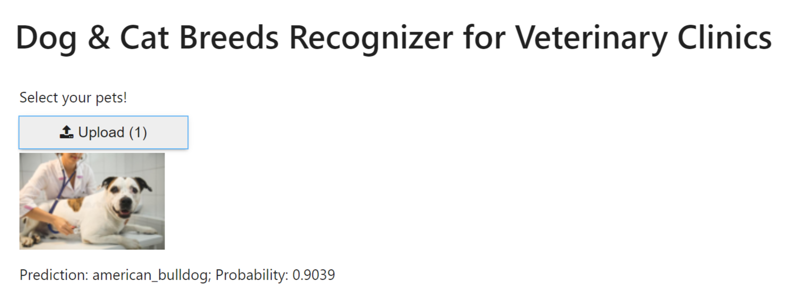
Version 1 of our "Dog & Cat Breeds Recognizer for Veterinary Clinics"
10. Turning your Web App into a startup product
This paragraph is written in the post Product based on a Deep Learning model (by fastai v2).