Problem 1 (20 pts)
(5 pts) Prove that $\mathrm{vec}(AXB) = (B^\top \otimes A)\, \mathrm{vec}(X)$ if $\mathrm{vec}(X)$ is a columnwise reshape of a matrix into a long vector. What does it change if the reshape is rowwise? Note: to make a columnwise reshape in Python one should use
np.reshape(X, order='f'), where the string'f'stands for the Fortran ordering.(5 pts) Let matrices $A$ and $B$ have eigendecompositions $A = S_A\Lambda_A S_A^{-1}$ and $B = S_B\Lambda_B S^{-1}_B$. Find eigenvectors and eigenvalues of the matrix $A\otimes I + I \otimes B$.
(10 pts) Let $A = \mathrm{diag}\left(\frac{1}{1000},\frac{1}{999},\dots \frac{1}{2}, 1, 1000 \right)$. Estimate analytically the number of iterations required to solve linear system with $A$ with the relative accuracy $10^{-4}$ using
- Richardson iteration with the optimal choice of parameter
- Chebyshev iteration
- Conjugate gradient method
Problem 2 (30 pts)
Spectral graph partitioning and inverse iteration
Given connected graph $G$ and its corresponding graph Laplacian matrix $L = D - A$ with eigenvalues $0=\lambda_1, \lambda_2, ..., \lambda_n$, where $D$ is its degree matrix and $A$ is its adjacency matrix, Fiedler vector is an eignevector correspondng to the second smallest eigenvalue $\lambda_2$ of $L$. Fiedler vector can be used for graph partitioning: positive values correspond to one part of a graph and negative values to another.
Inverse power method (15 pts)
To find the Fiedler vector we will use the inverse iteration with adaptive shifts (Rayleigh quotient iteration).
Write down the orthoprojection matrix on the space orthogonal to the eigenvector of $L$, corresponding to the eigenvalue $0$ and prove (analytically) that it is indeed an orthoprojection.
Implement the spectral partitioning as the function
partition:
# INPUT:
# A - adjacency matrix (scipy.sparse.csr_matrix)
# num_iter_fix - number of iterations with fixed shift (int)
# shift - (float number)
# num_iter_adapt - number of iterations with adaptive shift (int) -- Rayleigh quotient iteration steps
# x0 - initial guess (1D numpy.ndarray)
# OUTPUT:
# x - normalized Fiedler vector (1D numpy.ndarray)
# eigs - eigenvalue estimations at each step (1D numpy.ndarray)
# eps - relative tolerance (float)
def partition(A, shift, num_iter_fix, num_iter_adapt, x0, eps):  # 10 pts
    x = x0
    eigs = np.array([0])
    return x, eigs
Algorithm must halt before num_iter_fix + num_iter_adapt iterations if the following condition is satisfied $\|\lambda_k - \lambda_{k-1}\|_2 / \|\lambda_k\|_2 \leq \epsilon$ at some step $k$.
Do not forget to use the orthogonal projection from above in the iterative process to get the correct eigenvector.
It is also a good idea to use shift=0 before the adaptive stragy is used. This, however, is not possible since the matrix $L$ is singular, and sparse decompositions in scipy do not work in this case. Therefore, we first use a very small shift instead.
Generate a random
lollipop_graphusingnetworkxlibrary and find its partition. Draw this graph with vertices colored according to the partition.Start the method with a random initial guess
x0, setnum_iter_fix=0and comment why the method can converge to a wrong eigenvalue.
Stanford Bunny (15 pts)
Let us now find a partition of a large graph, obtained from the 3D model from The Stanford 3D Scanning Repository: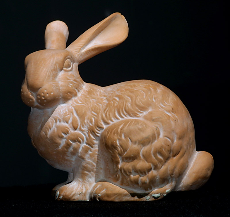
Install the trimesh library. In order to visualize 3D model smoothly you will also need to install
pygletlibrary (see trimesh instructions). Alternatively, you can draw and rotate model using 3D scatter inmatplotlibwith%matplotlib notebook.Download the 3D model of the bunny here.
You can read it and display with
mesh = trimesh.load(<path>)andmesh.show()respectively. Coordinates of the vertices and faces can be accessed withmesh.verticesandmesh.facesrespectively. Note that not every vertex is a part of a face, you should filter them out.Create an adjacency matrix of the graph corresponding to the mesh of the model (you can use
networkxlibrary for this). Verify that the number of connected components of the graph is exactly $1$.Find the "bunny" partitioning for
num_iter_fix=1, num_iter_adapt=2andnum_iter_fix=2, num_iter_adapt=10. Plot the convergence rate for the second case and discuss it. Draw 3D model with coloring according to the partitions. Withtrimeshyou can assign vertex colors asmesh.visual.vertex_colors[<vertex>] = (R,G,B,A).
Consider a 2D convection-diffusion equation in $\Omega = [0,1]^2$ $$ -\frac{\partial^2 u}{\partial x^2} - \frac{\partial^2 u}{\partial y^2} + \frac{\partial u}{\partial x} + \frac{\partial u}{\partial y} = f(x,y), \quad (x,y)\in \Omega $$ with zero Dirichlet boundary conditions $$ u_{\partial \Omega} = 0, $$ with known function $f(x,y)$ and unknown $u(x,y)$.
To find solution of this equation we will use the finite difference method. Standard second order finite difference discretization on a uniform grid $(x_i, y_j) = (ih, jh)$, $i,j = 0,\dots, N$, $h = \frac{1}{N}$ leads to the following system of equations: $$ \begin{split} &-\frac{u_{i+1,j} - 2u_{i,j} + u_{i-1,j}}{h^2} - \frac{u_{i,j+1} - 2u_{i,j} + u_{i,j-1}}{h^2} + \frac{u_{i+1, j} - u_{i,j}}{h} + \frac{u_{i, j+1} - u_{i,j}}{h} = f(ih, jh) \\ &u_{0,j} = u_{i,0} = u_{N,j} = u_{i,N} = 0, \quad i,j = 0,\dots,N, \end{split} $$
Write the system above as a matrix equation $BU_h + U_h C = F_h$ with matrices $U_h = \begin{bmatrix}u_{1,1} & \dots & u_{1,N-1} \\ \vdots & \ddots & \vdots \\ u_{N-1,1} & \dots & u_{N-1,N-1} \end{bmatrix}$, $F_h = \begin{bmatrix}f_{1,1} & \dots & f_{1,N-1} \\ \vdots & \ddots & \vdots \\ f_{N-1,1} & \dots & f_{N-1,N-1} \end{bmatrix}$. What are matrices $B$ and $C$?
Using Kronecker product properties rewrite analytically $ BU_h + U_h C = F_h$ as $A_h \mathrm{vec}(U_h) = \mathrm{vec}(F_h)$, where $\mathrm{vec}(\cdot)$ is a columnwise reshape.
What is matrix $A_h$?
- Choose $f(x,y) = 1$.
Solve the system with this $f$ using the scipy.sparse.linalg.spsolve which is direct sparse solver.
Use pandas library and print table that contains $N$ and time of solving for $N=127, 255, 511$.
Matrices $B, C$ and $A_h$ should be assembled in the CSR format using functions from the scipy.sparse package (functions scipy.sparse.kron and scipy.sparse.spdiags will be helpful). Do not use full matrices! Use only sparse arithmetics.
# INPUT - dimension of the grid along the one side of the square
# OUTPUT - matrix Ah for 2D convection-diffusion problem in CSR sparse format
def build_matrix(N):  # 5 pts
    # Your code is here
    return A
Fix initial random guess $x_0$, maximal number of iterations and required tolerance. These parameters will be the same for all iterative methods that you will test
Run
cg,minres,GMRES,BicgStabfromscipy.sparse.linalgpackage with generated matrix for 2D convection-diffusion equation, right-hand side $f(x, y) = 1$ and above described parameters.What are the iterative methods diverge and why?
What are the iterative methods of choice? Explain why.
Plot the relative residual norm $\frac{\|Ax_k - f\|_2}{\|f\|_2}$ w.r.t number of iteration and w.r.t elapsed time. Assume that every iteration lasts the same number of seconds
Run the methods of choice with and without ILU0 preconditioner (use it from
scipy.sparsepackage) and Block Jacobi preconditioner for $N=256$. You should implement Block Jacobi preconditioner in the most efficient manner, in particular the most complex operation is solve linear systems with $N \times N$ matrix and multiple right-hand sides. Plot relative error w.r.t iteration number for both cases and for both preconditioners on one plot. Don't forget add legend. Also plot relative error w.r.t time in the similar way. Assume that every iteration lasts the same number of seconds
Problem 4 (30 pts)
Again QR, oh no!
<img src='qrcode.jpg', width=300px>
- In this problem you asked to find the convolution of the $n\times n$, $n=512$ QR(-code) with the following filter
using FFT.
* Write function matvec that produces multiplication of $T$ by a given vector $x$.
* Use scipy.sparse.linalg.LinearOperator to create an object that has attribute .dot() (this object will be further used in the iterative process). Note that .dot() input and output must be 1D vectors, so do not forget to use reshape.
* Convolve qrcode.jpg with $T$ for $\alpha = \frac{1}{100}$.Plot the result as an image.
* What is the complexity of this operation?
*
Note: You can use standart FFT, from e.q. numpy.fft
Run an appropriate Krylov method(s) with the obtained Linear Operator and try to reconstruct back QR-code using the right-hand side from the first bullet (smoothed QR-code).
On one figure plot norm of residual with respect to the number of iterations for $\alpha = \{\frac{1}{50},~~\frac{1}{100},~~\frac{1}{200}\}$ and corresponding right hand side. Comment on the results.
Bonus: Find image
noisy_extra.jpgin the attached to this problem set file. This image is the QR-code with the beautiful message, convolved with $T$, parameter $\alpha=\frac{1}{100}$ plus small random noise:
<img src='noisy_extra.jpg', width=300px> * Your goal now is to get the link from the image. Since the problem is very ill-posed you need some regularization, denoising or anything else.
#Function that will be provided into scipy.sparse.linalg.LinearOperator
#INPUT:  1D array %vec and
#        alpha with default value==1/100.
#OUTPUT: 1D array
#Hint: you can vary alpha using lambda function as argument of linalg.LinearOperator:
#                                                     e.q.   lambda x: matvec(x,1/50.)
def matvec(vec, alpha=1/100.):  # 15 pts
    return out