Introduction
This notebook is based on my previous attempt with the GTD. At that time I explored the dataset and tried to start running ML models on it. In this round, on the other hand, first, I tried to reconstruct two recent papers 'by hand' written on the same problem, that is, the prediction of terrorist groups based on the characteristics of previous incidents. While I managed to build out their preprocessing and modeling environment I could not do it perfectly because
- The papers do not describe every single step in their workflow
- Both groups of authors used WEKA with its own in-built algorithms (and did not publish their code). For instance, one of them used the J48 model which is an Java implementation of the C4.5 (while sklearn uses CART).
After going through the papers, I started to build out a pipeline which I hoped will allow me to turn on/off various features on the whole data processing/modeling workflow. One of my main reason for that was to examine the relationship of the way the initial problem is framed to modelling.
Problem discussion
To give an example, the problem of predicting perpetrator groups is meant in a number of different ways mirroring the specific issue the modelers want to solve and the means they have for that. Both papers (and most of the earlier ones) describe cases where the problem was narrowed down to pedict Indian cases and usually with a general idea of helping to find out the groups behind an incident and eventually to arrest the perpetrators. This can imply many things (perhaps most importantly that there is an agent who can relatively quickly collect the same information a model is based on). Accordingly, the particular model setting needs to mirror this situation (i.e. what features do we allow into the model, how do we clean the data, where do we split, etc.). Finally, this is also related to the issue of those types of data leaking problems where models take into account 'information from the future'.
To examine this, however, I wanted to create a working flow which allows me to look over the whole process and to turn particular features on/off in it. Unfortunately, scikit-learn's current Pipeline (as far as I understand) does not allow
- tranformations based on label values,
- changing sample size witin the pipeline
- building the test-train split into the pipeline (or maybe I just did not find out how to do it..)
To tackle this issue I created a CustomTransformation wrapper around the normal scikit-learn entities and hoped that I can pass label and other information between the steps so they also allow me to include the above mentioned features. This, however, proved to be harder than I expected (e.g. I have not used classes before) so after a couple of days I had to give up this project to rather focus on the actual prediction problem.
This notebook
In this notebook then I connected the aims and some of the functions of the previous ones together. Here, I continued to recreate the papers, but now I also tried to build out if not a pipeline but a workflow to see what affects what. Even in this way, it was not entirely easy to understand which step should come before/after another, so at one some I summarized it both in text and graph which you can find at the end of this notebook.
Eventually, I ran a number of modelling situations which gave me an insight about the the issues around the paper although I did not go into either hyperparameter selection, metric interpretation (or even to use multiple metrics) or multilabel classification (which I hoped to do at this round).
The papers
CHRIST
D. Talreja, J. Nagaraj, N. J. Varsha and K. Mahesh, "Terrorism analytics: Learning to predict the perpetrator," 2017 International Conference on Advances in Computing, Communications and Informatics (ICACCI), Udupi, 2017, pp. 1723-1726. doi: 10.1109/ICACCI.2017.8126092
KAnOE
Varun Teja Gundabathula and V. Vaidhehi, An Efficient Modelling of Terrorist Groups in India using Machine Learning Algorithms, Indian Journal of Science and Technology, Vol 11(15), DOI: 10.17485/ijst/2018/v11i15/121766, April 2018
Libraries
Versions
- pandas: 0.23.3
- scikit-learn: 0.19.1
- numpy: 1.15.0
- scipy: 1.1.0
- imblearn 0.0
Warning control
import warnings

warnings.filterwarnings(action='ignore', category=DeprecationWarning)
warnings.filterwarnings(action='ignore', category=FutureWarning)
Data handling
import pandas as pd
import numpy as np
Preprocessing
from sklearn.preprocessing import LabelEncoder, FunctionTransformer, Imputer, StandardScaler, Normalizer
from sklearn.feature_selection import SelectKBest, chi2, RFE
from imblearn.over_sampling import SMOTE, RandomOverSampler
from scipy.sparse import csr_matrix
Pipeline
from sklearn.pipeline import Pipeline
from sklearn.model_selection import train_test_split, KFold, cross_val_score, cross_validate, \
    StratifiedKFold
Models
from sklearn.tree import DecisionTreeClassifier
from sklearn.neighbors import KNeighborsClassifier
from sklearn.svm import LinearSVC
from sklearn.linear_model import LogisticRegression,
from sklearn.ensemble import ExtraTreesClassifier, RandomForestClassifier
from sklearn.naive_bayes import GaussianNB
/home/andras/anaconda3/lib/python3.6/site-packages/sklearn/ensemble/weight_boosting.py:29: DeprecationWarning: numpy.core.umath_tests is an internal NumPy module and should not be imported. It will be removed in a future NumPy release.
  from numpy.core.umath_tests import inner1d
Metrics
from sklearn.metrics import accuracy_score, precision_score, classification_report, roc_auc_score
Utilities
import time
# This sets the temp folder and is required for "jobs=-1" to work on Kaggle at some cases
# (see https://www.kaggle.com/getting-started/45288#292143)
%env JOBLIB_TEMP_FOLDER=/tmp
env: JOBLIB_TEMP_FOLDER=/tmp
Loading the data
Previously we loaded the data and created a sample out of it. From now on we are going to use it for our analysis and modeling.
# Instead of the excel from their homepage, I use the csv version they uploaded to Kaggle
# gtd = pd.read_excel("globalterrorismdb_0617dist.xlsx")
gtd = pd.read_csv("../input/globalterrorismdb_0617dist.csv", encoding='ISO-8859-1')
/home/andras/anaconda3/lib/python3.6/site-packages/IPython/core/interactiveshell.py:2785: DtypeWarning: Columns (4,6,31,33,53,61,62,63,76,79,90,92,94,96,114,115,121) have mixed types. Specify dtype option on import or set low_memory=False.
  interactivity=interactivity, compiler=compiler, result=result)
# In case we want to use a sample
# gtd_ori = gtd
gtd = gtd.sample(frac=0.1)
Recreating the CHRIST paper
The authors of the paper trained and tested the model on a subsample of the whole dataset, namely:
- Between 1970-2015
- Incidents related to India
- Cases to which the dataset attributes a perpetrator group (i.e. no 'Unknown' labels)
They also preselected a number of features for the model which they used.
Defining the steps
Handling missing values
There are a number of features where missing values are noted with a special code.
miscodes = {"0": ['imonth', 'iday'],
            "-9": ['claim2', 'claimed', 'compclaim', 'doubtterr', 'INT_ANY', 'INT_IDEO', 'INT_LOG', 'INT_MISC',
                   'ishostkid', 'ndays', 'nhostkid', 'nhostkidus', 'nhours', 'nperpcap', 'nperps', 'nreleased',
                   'property', 'ransom', 'ransomamt', 'ransomamtus', 'ransompaid', 'ransompaidus', 'vicinity'],
            "-99": ['ransompaid', 'nperpcap', 'compclaim', 'nreleased', 'nperps', 'nhostkidus', 'ransomamtus',
                    'ransomamt', 'nhours', 'ndays', 'propvalue', 'ransompaidus', 'nhostkid']}
def mistonan(data, nancode):
    """Replaces columns' missing value code with numpy.NaN.

    Parameters:
    `data`: dataframe

    `nanvalue` : the code of the missing value in the columns
    """
    data=data.copy()

    for code in nancode.keys():
        for col in nancode[code]:
            if col in data.columns:
                data.loc[:, col].where(data.loc[:, col] != float(code), np.NaN, inplace=True)

    return data
tdat = gtd.copy()
tdat[tdat == -9].count().sum() #The number of '-9' values in the test data
29645
tdat.isna().mean().mean() # The mean ratio of missing values over the columns
0.5674261052951983
The function replaces the codes with NaNs
tdat = mistonan(tdat, miscodes)
tdat[tdat == -9].count().sum()
1
tdat.isna().mean().mean()
0.5851838806813858
Imputing missing values
def nanimputer(dat):
    """Imputes missing values with the column's mean
    Takes:
        'dat', dataframe

    Returns:
        'tdat': the dataframe with the imputed values
    """
    tdat = dat.copy()
    numcols = tdat.select_dtypes(exclude=object).columns # numeric columns
    hasna = tdat[numcols].isna().any() # query about missing values
    hasnacols = hasna[hasna].index # columns w/ missing values

    # A simple conditional imputer converted to df
    tdat[hasnacols] = pd.DataFrame(np.where(tdat[hasnacols].isna(),
                                            tdat[hasnacols].mean(),
                                            tdat[hasnacols]),
                                   columns=tdat[hasnacols].columns,
                                   index=tdat[hasnacols].index)

    return tdat
The missing value ratio in columns before and after the transformation
tdat.select_dtypes(exclude=object).isna().mean().sort_values(ascending=False)
weapsubtype4      0.999765
weaptype4         0.999706
claimmode3        0.999061
guncertain3       0.998004
claim3            0.997945
ransompaid        0.997887
attacktype3       0.997652
ransompaidus      0.997593
ransomamtus       0.997417
claimmode2        0.996947
ransomamt         0.994071
targsubtype3      0.993425
natlty3           0.993073
targtype3         0.993014
compclaim         0.992427
weapsubtype3      0.991136
weaptype3         0.990431
claim2            0.989727
guncertain2       0.989257
nhours            0.988612
ndays             0.981626
nreleased         0.966481
attacktype2       0.966246
hostkidoutcome    0.944232
targsubtype2      0.940475
propvalue         0.940006
natlty2           0.940006
targtype2         0.937951
weapsubtype2      0.936190
nhostkid          0.935721
                    ...
weapsubtype1      0.109657
nwound            0.090167
doubtterr         0.082301
nkill             0.056355
targsubtype1      0.053009
latitude          0.025125
longitude         0.025125
natlty1           0.007455
iday              0.004755
ishostkid         0.003053
INT_MISC          0.002818
guncertain1       0.002172
vicinity          0.000176
imonth            0.000117
extended          0.000000
country           0.000000
region            0.000000
iyear             0.000000
specificity       0.000000
suicide           0.000000
crit1             0.000000
crit2             0.000000
crit3             0.000000
multiple          0.000000
success           0.000000
attacktype1       0.000000
targtype1         0.000000
weaptype1         0.000000
individual        0.000000
eventid           0.000000
Length: 77, dtype: float64
tdat = nanimputer(tdat)
tdat.select_dtypes(exclude=object).isna().mean().sort_values(ascending=False)
INT_ANY           0.0
natlty2           0.0
attacktype2       0.0
attacktype3       0.0
targtype1         0.0
targsubtype1      0.0
natlty1           0.0
targtype2         0.0
targsubtype2      0.0
targtype3         0.0
claimed           0.0
targsubtype3      0.0
natlty3           0.0
guncertain1       0.0
guncertain2       0.0
guncertain3       0.0
individual        0.0
nperps            0.0
attacktype1       0.0
suicide           0.0
success           0.0
multiple          0.0
iyear             0.0
imonth            0.0
iday              0.0
extended          0.0
country           0.0
region            0.0
latitude          0.0
longitude         0.0
                 ...
ndays             0.0
ransomamt         0.0
claim2            0.0
ransomamtus       0.0
ransompaid        0.0
ransompaidus      0.0
hostkidoutcome    0.0
nreleased         0.0
INT_LOG           0.0
INT_IDEO          0.0
property          0.0
nwoundte          0.0
nwoundus          0.0
nwound            0.0
claimmode2        0.0
claim3            0.0
claimmode3        0.0
compclaim         0.0
weaptype1         0.0
weapsubtype1      0.0
weaptype2         0.0
weapsubtype2      0.0
weaptype3         0.0
weapsubtype3      0.0
weaptype4         0.0
weapsubtype4      0.0
nkill             0.0
nkillus           0.0
nkillter          0.0
eventid           0.0
Length: 77, dtype: float64
The mean as a new value in the column. I just realized that this interferes with the datatype coverter function (see below).
tdat.nwoundte.value_counts()
0.000000     9915
0.100563     6902
1.000000       90
2.000000       33
3.000000       21
4.000000       13
9.000000        8
10.000000       7
6.000000        7
7.000000        6
8.000000        6
5.000000        5
13.000000       3
15.000000       3
50.000000       2
14.000000       2
24.000000       2
20.000000       2
11.000000       2
18.000000       1
12.000000       1
17.000000       1
19.000000       1
38.000000       1
23.000000       1
Name: nwoundte, dtype: int64
I tried to use this built-in sklearn version but it provided me a numpy array without indexes which I found hard to transfer back.
#def imputenans(data,  misvals=None, strategy='median'):
#    if len(misvals) == 0:
#        return data
#
#    misdat = data.copy()
#    impute = Imputer(missing_values=misvals[0],
#                     strategy=strategy,
#                     verbose=0)
#
#    numcols = misdat.select_dtypes(exclude=[object]).columns
#    #numeric = misdat.copy().loc[:, numcols]
#
#    misdat.loc[:, numcols] = pd.DataFrame(impute.fit_transform(misdat.loc[:, numcols]))
#
#    return imputenans(misdat, misvals=misvals[1:], strategy=strategy)
Sampling based on attribute values
def attribute_sampler(X, startdate, enddate, country=None):
    """Filters data samples based on the values of the attributes
    Here I tried to separate those transformations which are not related
    to the label.

    Takes
    - X: dataframe
    - startdate and enddate: first and last year to include
    - country: the countries to include
    """
    if 'country_txt' in X.columns:
        if country == None:
            country = X.country_txt
        else:
            X = X[X.country_txt == country]

    filcrit = (X.iyear >= max(startdate, X.iyear.min())) \
            & (X.iyear <= min(enddate, X.iyear.max()))

    return X[filcrit]
Initially (within this notebook) I also converted the functions with FunctionTransfromer into possible pipeline steps but finally I did not use them.
attsamp = FunctionTransformer(attribute_sampler,
                              validate=False,
                              kw_args={
                                  'startdate': 1970,
                                  'enddate': 2015,
                                  'country': 'India'
                             })
tX0 = attsamp.fit_transform(tdat).copy()
ty0 = tdat.gname[tX0.index]
# Checks
print(tX0.iyear.min(), tX0.iyear.max())
print(tdat.reindex(tX0.index).country_txt.unique()[0])
1979 2015
India
Selecting columns
def col_sel(X, columns=None):
    """Selects columns from a DataFrame based on a list of column names.
    Takes
    - X: DataFrame
    - columns: list of column names

    Returns
    - X: The DataFrame with the filtered columns
    """
    if columns != None:
        X = X.loc[:, columns]


    return X
# The two set of colums the two papers used in their model
kanoe_cols = ['iyear', 'attacktype1', 'targtype1', 'targsubtype1', 'weaptype1',
              'latitude', 'longitude', 'natlty1', 'property', 'INT_ANY', 'multiple', 'crit3']

christ_cols = ['iyear', 'imonth', 'iday', 'extended', 'provstate', 'city', 'attacktype1_txt',
               'targtype1_txt',  'nperps', 'weaptype1_txt', 'nkill', 'nwound', 'nhostkid']
colsamp = FunctionTransformer(
    col_sel,
    validate=False,
    kw_args={'columns': christ_cols}) # the another option: kanoe_cols
tX0 = colsamp.fit_transform(tX0)
# Check
print(tX0.columns.values)
['iyear' 'imonth' 'iday' 'extended' 'provstate' 'city' 'attacktype1_txt'
 'targtype1_txt' 'nperps' 'weaptype1_txt' 'nkill' 'nwound' 'nhostkid']
Sampling based on target values
def target_sampler(X, y, mininc, onlyknown=True, ukcode='Unknown'):
    """Samples both X and y based on information from y
    (as opposed to for instance the attribute sampler
    which relies only on information from X)

    Takes:
    - X, y: The attributes and their labels
    - mininc: The minimum occurance of a label to include
    (i.e. for how many incidents a group is responsible)
    - onlyknown: whether to drop samples with unknown target values
    - ukcode: the code for unknown targets (this can be different if we
    encode the labels)

    Returns
    - X
    """

    if onlyknown: # Check for known labels and filter the data
        nukcrit = y != ukcode
        X = X[nukcrit]
        y = y[nukcrit]

    # Maps the labels with the minimum required occurences
    mininc = y.isin(y.value_counts() \
                    [y.value_counts() >= mininc] \
                    .index.values)

    return X[mininc] # y is missing from here!
After the transformation the data has no 'Unknown' values and the minimum frequency of included labels is 2.
tX1 = target_sampler(tX0, ty0, mininc=2, onlyknown=True, ukcode='Unknown')
ty1 = ty0[tX1.index]
# Checks
print(tX1.shape[0] == ty1.shape[0])
print(('Communist Party of India - Maoist (CPI-Maoist)' == ty1).any())
print(('Unknown' != ty1).all())
print(ty1.value_counts().min())
True
True
True
2
New feature creation
def naff(X, crits, zeroval, newcol):
    """ A function which creates a new feature based on the number
    of killed, wounded and hostages taken in an incident.
    It also fills zero values at some of the places.
    It basically bins the columns into categories based on effect size
    and provides a column of their combinations sets.

    Takes
    -X: The Dataframe to transform
    -crits, dict: the criteria based on which the new feature is created.

    It works with the following structure:
     {'nkill': (62, 124, 'abc')
         - the key is the column name
         - the first two values are numeric thresholds based on which
         it bins the feature
         - the three-letter string are the three codes each bin receives as a code

    -zeroval: the code zero values receive
    -newcol: the name of the new column

    """
    # Technical column
    n = pd.Series('_')

    # The loops go over the columns and bin them
    for key, i in zip(crits.keys(), range(len(crits))):

        # I start with creating a series of 'n'-s with the
        # indexes of the dataframe
        i = pd.Series('n', name=key).repeat(X.shape[0])
        i.index = X.index

        # Binning the column based on the criteria from the dict
        i[(X.loc[:,key] > 0)
          & (X.loc[:,key] < crits[key][0])] = crits[key][2][2]
        i[(X.loc[:,key] <= crits[key][1])
          & (X.loc[:,key] >= crits[key][0])] = crits[key][2][1]
        i[X.loc[:,key] > crits[key][1]] = crits[key][2][0]

        # Concatenating the new column to the technical/other columns
        n = pd.concat((n, i), axis=1)

    # Cleaning missing values
    n.nhostkid[n.nhostkid == -99] = zeroval
    n = n.replace(np.NaN, zeroval)

    # Dropping the technical column
    n = n.reindex(X.index).drop(columns=0)

    # Merging the values of the three columns together into strings
    n = n.iloc[:,0] +  n.iloc[:,1] +  n.iloc[:,2]

    # Replacing the old columns with the new one
    X = X.drop(columns=list(crits.keys()))
    X[newcol] = n

    # Further data cleaning
    X.nperps = X.nperps.where(X.nperps != -99, 0)
    X.nperps = X.nperps.fillna(0)

    return X
The feature creation criteria
'crits' : {'nkill': (62, 124, 'abc'),
           'nwound': (272, 544, 'def'),
           'nhostkid': (400, 800, 'ghi')},
'zeroval': 'n',
'newcol': 'naffect'
naff_col = FunctionTransformer(naff,
                               validate=False,
                               kw_args={'crits' : {'nkill': (62, 124, 'abc'),
                                                'nwound': (272, 544, 'def'),
                                                'nhostkid': (400, 800, 'ghi')},
                                        'zeroval': 'n',
                                        'newcol': 'naffect'
                                      })
The new column after the tranformation
tX2 = naff_col.fit_transform(tX1).copy()
pd.concat((tX1.loc[:, ['nkill', 'nwound', 'nhostkid']], tX2.naffect), axis=1).head()
| nkill | nwound | nhostkid | naffect | |
|---|---|---|---|---|
| 123631 | 1.0 | 0.0 | 9.881279 | cni |
| 34826 | 7.0 | 60.0 | 9.881279 | cfi |
| 100820 | 3.0 | 4.0 | 9.881279 | cfi |
| 75164 | 0.0 | 0.0 | 9.881279 | nni |
| 59111 | 0.0 | 0.0 | 9.881279 | nni |
Checks (for an earlier version) does not work at the moment
# crits : {'nkill': (62, 124, 'abc'),
#          'nwound': (272, 544, 'def'),
#          'nhostkid': (400, 800, 'ghi')}
#
# print((((X.loc[:, crits.keys()] == 0)
#         | (X.loc[:, crits.keys()] == -99)
#        ) == (naffect == 'n')).all().all())
#
# print(((X.loc[:, crits.keys()] > crits[key][1]) == (nc.isin(('a', 'd', 'g')))).all().all())
#
# print((((X.loc[:, crits.keys()] <= crits[key][1])
#         & (X.loc[:, crits.keys()] >= crits[key][0])
#        ) == (nc.isin(('b', 'e', 'h')))).all().all())
#
# print((((X.loc[:, crits.keys()] < crits[key][0])
#         & (X.loc[:, crits.keys()] > 0)
#        ) == (nc.isin(('c', 'f', 'i')))).all().all())
#
# print((tX2 != -99).all().all())
# print(~tX2.isna().any().any())
Setting the colum datatypes
df = gtd.copy()
def dtypeconv(df, col_dt_dict=None, auto=True):
    """Converts a DataFrame's datatype based on either a dictionary
    or an automatic logic.
    ** The automatic mode is unfinished and probably interfers with the data imputer **

    Takes
    - df: Dataframe to transform
    - col_dt_dict; the dict of {'column': 'intended datatype'} pairs
    - auto, Boolean: if True, the function ignores the dict and follows the
    automatic logic.

    Returns the transformed dataframe

    The automatic coverter logic
    This is currently limited and probably has some dangers I am not unaware of but,
    I think, it help with the speed of models. It can do the following things:
    - Converts objects to categoricals for those columns where the ratio
    of unique labels are less than 0.5.
    - Downcasts unsigned integer values into the lowest possible category
    (e.g. uint8 for columns with only binary values)
    """

    df = df.copy()

    if auto == True:
        objcidx = df.select_dtypes(object).columns # Indexes of object type columns
        numcidx = df.select_dtypes(exclude=object).columns # Indexes of numerical columns
        nnegcidx = numcidx[(df[numcidx] >= 0).all()] # Indexes of non-negative columns

        # Converting objects to categoricals
        if len(objcidx) != 0:
            unqrat = (df.nunique() / df.count()) # Unique value ratio
            lehalfun = unqrat[unqrat < 0.5].index # Columns with less than 0.5 unique ratio
            df[objcidx & lehalfun] = df[objcidx & lehalfun].astype('category')


        # Downcasting integers
        # Checks for actual whole values
        # (During writing up this I realized that it interferes with the
        # imputer function)

        # Indexes of columns with zero fractional modulus 1
        tointidx = nnegcidx[(df[nnegcidx] % 1).max() == 0]
        icolmaxes = df[tointidx].max() # Their maximum values

        # Distributing the column names
        ui8idx = tointidx[(icolmaxes <= 255)]
        ui16idx = tointidx[(icolmaxes > 255) & (icolmaxes <= 65535)]
        ui32idx = tointidx[(icolmaxes > 65535) & (icolmaxes <= 4294967295)]
        ui64idx = tointidx[(icolmaxes > 4294967295)]

        df[ui8idx] = df[ui8idx].astype('uint8')
        df[ui16idx] = df[ui16idx].astype('uint16')
        df[ui32idx] = df[ui32idx].astype('uint32')
        df[ui64idx] = df[ui64idx].astype('uint64')

        return df

    else:
        # Dictionary-based dtype conversion
        dks = col_dt_dict.keys() # Keys

        if len(tuple(dks)) == 0:
            return df

        dtype = tuple(dks)[0] # Type stored as key
        cols = col_dt_dict[dtype] # Columns

        # We can also provide a datatype instead of a column name
        # so it will transform all the columns of that type
        if type(cols) == type:
            cols = df.select_dtypes(cols).columns.values

        df.loc[:, cols]= df.loc[:, cols].astype(dtype)

        # Tempdic allowing us recursion
        tempdict = col_dt_dict.copy()
        del tempdict[dtype]

        return dtypeconv(df, tempdict)
Used dtype transformations
'col_dt_dict' : {'int8': ('imonth', 'iday', 'extended'),
                 'int16': ('iyear', 'nperps'),
                 'category': object}
dtconv = FunctionTransformer(dtypeconv,
                             validate=False,
                             kw_args={'auto' : False,
                                      'col_dt_dict' : {'int8': ('imonth', 'iday', 'extended'),
                                                       'int16': ('iyear'),
                                                       'category': object}
                                     })
Old and new datatypes
tX2.dtypes
iyear                int64
imonth             float64
iday               float64
extended             int64
provstate           object
city                object
attacktype1_txt     object
targtype1_txt       object
nperps             float64
weaptype1_txt       object
naffect             object
dtype: object
tX3 = dtconv.fit_transform(tX2)
ty3 = ty0[tX3.index]
tX3.dtypes
iyear                uint16
imonth                uint8
iday                  uint8
extended              uint8
provstate          category
city                 object
attacktype1_txt    category
targtype1_txt      category
nperps              float64
weaptype1_txt      category
naffect            category
dtype: object
Automatic conversion
dtypeconv(tX2, auto=True).dtypes
iyear                uint16
imonth                uint8
iday                float64
extended              uint8
provstate          category
city                 object
attacktype1_txt    category
targtype1_txt      category
nperps              float64
weaptype1_txt      category
naffect            category
dtype: object
As it turns out, the two does not provide the same results, because there might be fractional values where they should not be (in this case, the calendar day of the incident perhaps due to the imputation above)
tX3.dtypes == dtypeconv(tX2, auto=True).dtypes
iyear               True
imonth              True
iday               False
extended            True
provstate           True
city                True
attacktype1_txt     True
targtype1_txt       True
nperps              True
weaptype1_txt       True
naffect             True
dtype: bool
(tX2.iday % 1)[(tX2.iday % 1) > 0]
103627    0.634246
102826    0.634246
Name: iday, dtype: float64
Encoding categoricals
X values
def catenc(X, sparse=False):
    """Uses pandas.get_dummies to create binary columns
    from the values of the object or category type attributes.

    Takes
    X: the dataframe to transform
    sparse: if True, transforms the dataframe to sparse at the end

    Returns the dataframe
    """

    X = pd.get_dummies(X)
    #cols = X.columns

    if sparse:
        X = csr_matrix(X)

    return X #, cols
codeX = FunctionTransformer(catenc, validate=False, kw_args={'sparse': False})
tX4 = codeX.fit_transform(tX3)
y values
def lenc(labels, labelencoder=None, inv=False):
    """
    Encoding label values with scikit-learn's LabelEncoder.

    Takes
    - labels, array or Series of labels to encode
    - labelencoder, the encoder function (needed when
    doing recoding)
    - inv, boolean: If True, does inverse encoding (recoding). It requires the
    encoder function as imput to work.

    Returns
    - l: the encoded labels as pandas.Series
    - lec: the encoding function (for later recoding)
    - miscode: the code for the 'Unknown' value
    """
    l = labels.copy()

    # Inverse encoding
    if inv == True:
        l = labelencoder.inverse_transform(l)
        l = pd.Series(l) # Transform to series
        l.index = labels.index
        return l

    else:
        lec = LabelEncoder()
        l = lec.fit_transform(l)

        # I transfer back the labels to series so I sample it with
        # X transformations based on its indexes
        l = pd.Series(l)
        l.index = labels.index

        # Returning the code of the "Unknown" label value
        if 'Unknown' in labels.values:
            miscode = np.unique(l[labels == 'Unknown'])[0]
            return l, lec, miscode
        else:
            return l, lec, None
- The new codes
- The code of the 'Unknown' label
- The result of recoding
l, lec, unkonwn_code = lenc(ty3)
print(l[:10])
print(unkonwn_code)
print(lenc(labels=l, labelencoder=lec, inv=True)[:10])
123631    38
34826     49
100820    18
75164     49
59111     27
133710    24
111255    33
94076      4
93803      4
96486      4
dtype: int64
None
123631                   People's Liberation Front of India
34826               United Liberation Front of Assam (ULFA)
100820              Karbi People's Liberation Tigers (KPLT)
75164               United Liberation Front of Assam (ULFA)
59111                                    Muslim Separatists
133710                                              Maoists
111255    National Socialist Council of Nagaland-Isak-Mu...
94076        Communist Party of India - Maoist (CPI-Maoist)
93803        Communist Party of India - Maoist (CPI-Maoist)
96486        Communist Party of India - Maoist (CPI-Maoist)
dtype: object
/home/andras/anaconda3/lib/python3.6/site-packages/sklearn/preprocessing/label.py:151: DeprecationWarning: The truth value of an empty array is ambiguous. Returning False, but in future this will result in an error. Use `array.size > 0` to check that an array is not empty.
  if diff:
ency = FunctionTransformer(lenc, validate=False)
ty4, tlec, tukcode = ency.fit_transform(ty3)
# Checks
print(np.unique(ty4).size == ty3.nunique())
True
Transforming X into sparse form
This is a common step in the workflow, so I put it here
tX4 = csr_matrix(tX4)
(tX4.toarray()[:,0] == tX3.iloc[:,0]).all()
True
Rebalancing
The authors of the CHRIST paper used SMOTE overbalancing and mixed balancing. Because at first it was slow I focused only on overbalancing (because that created the best results for them).
EDIT: actually 'all' does mixed sampling, which I used because 'minorty' only oversamples the less frequent labels which in a multi class case are not all infrequent ones.
smote = SMOTE(ratio='all', k_neighbors=1, n_jobs=-1)
%%time
tX5, ty5 = smote.fit_sample(tX4, ty4)
CPU times: user 10.8 s, sys: 2.42 s, total: 13.2 s
Wall time: 20 s
The new nuber of samples
# Checks
print(tX5.shape)
print(ty5.shape)
print((pd.Series(ty5).value_counts() == pd.Series(ty4).value_counts().max()).all())
(7072, 445)
(7072,)
True
Prediction
Splitting the dataset
validation_size = 0.2
seed = 17
# The authors focused only on incidents from India.
atts = gtd[gtd.country_txt == 'India'].copy()
labels, LEC, ukcode = lenc(labels=atts.gname)
X_train, X_test, y_train, y_test = train_test_split(atts.drop(columns='gname'),
                                                    labels,
                                                    test_size=validation_size,
                                                    random_state=seed)

# Storing the original values for technical checks
X_train0, X_test0, y_train0, y_test0 = X_train.copy(), X_test.copy(), y_train.copy(), y_test.copy()

print(X_train.shape)
print(X_test.shape)
print(y_train.shape)
print(y_test.shape)
(821, 134)
(206, 134)
(821,)
(206,)
Preprocessing
The following function gathers together the previous steps.
def preproc(X_train, y_train,
            startdate=1970, enddate=2016,
            country=None,
            ukcode='Unknown', onlyknown=False, mininc=1,
            misctona=True, maxna=0, impute=False, nadrop=False,
            dropspec=True,
            onlyprim=True):
    """
    A wrapper function collecting many of the data processing steps.

    Takes
    - X_train, y_train
    - startdate, enddate

    - country

    - ukcode, string of numeric: the code of the unknown target label

    - onlyknown: if True, samples with 'unknown' (or what is defined by `ukcode`) labels are excluded

    - mininc, int: labels with minimum frequency to include

    - misctona, bool: if True, transforms the missing codes into nans

    - maxna, float: the minimum ratio (between 0 and 1) of allowed missing values in a column,
    e.g. 0.05 means that columns with more than 95% of missing values are excluded

    - impute, bool: if True, imputes mean values into the missing ones

    - nadrop, bool: if True, drops samples with missing values
    (after dropping the columns and imputation)

    - dropspec, bool: if True drops special columns

    - onlyprim, bool: if True, drops secondary and tertiary groups and all subnames.

    Returns
    X_train, y_train
    """

    # drops special columns
    if dropspec == True:
        X_train = X_train.drop([
            'eventid',
            'addnotes',
            'scite1',
            'scite2',
            'scite3',
            'dbsource'],
            axis=1,
            errors='ignore')

    # leaving only the primary label values
    if onlyprim == True:
        X_train = X_train.drop(columns=['gsubname',
                                        'gname2',
                                        'gsubname2',
                                        'gname3',
                                        'gsubname3'],
                               axis=1,
                               errors='ignore')

    # Sampling based on attribute values only
    X_train = attribute_sampler(X_train,
                                startdate=startdate,
                                enddate=enddate,
                                country=country)

    # Original missing codes to replace with np.NaN
    if misctona == True:
        miscodes = {"0": ['imonth', 'iday'],
                "-9": ['claim2', 'claimed', 'compclaim', 'doubtterr', 'INT_ANY', 'INT_IDEO', 'INT_LOG', 'INT_MISC',
                       'ishostkid', 'ndays', 'nhostkid', 'nhostkidus', 'nhours', 'nperpcap', 'nperps', 'nreleased',
                       'property', 'ransom', 'ransomamt', 'ransomamtus', 'ransompaid', 'ransompaidus', 'vicinity'],
                "-99": ['ransompaid', 'nperpcap', 'compclaim', 'nreleased', 'nperps', 'nhostkidus', 'ransomamtus',
                        'ransomamt', 'nhours', 'ndays', 'propvalue', 'ransompaidus', 'nhostkid']}

        X_train = mistonan(X_train, miscodes)

    # Dropping columns beyond a threshold of missing value ratios
    if maxna != 0:
        X_train = X_train.dropna(axis=1, thresh=X_train.shape[0] * (1 - maxna))

    # Imputing missing values
    if impute == True:
        X_train = nanimputer(X_train)

    # Dropping samples with missing values
    if nadrop == True:
        X_train = X_train.dropna()


    # We need to sample `y_train` because the next transformation
    # requires both x and y to be of the same sample size
    # -- possibly this was required for an earlier version
    y_train = y_train[X_train.index]
    X_train = target_sampler(X_train, y_train,
                             mininc=mininc,
                             onlyknown=onlyknown,
                             ukcode=ukcode)

    # We sample `y_train` again to mirror the previous X transformations
    y_train = y_train[X_train.index]

    return X_train, y_train
The set parameters (based on the paper):
- Only samples with known labels
- Only labels with minimum 2 occurences
X_train, y_train = preproc(
    X_train, y_train,
    onlyknown=True,
    ukcode=ukcode,
    mininc=2,
    maxna=0.05,
    nadrop=True # They do not mention handling missing values, so I simply drop the samples
)
Selecting the proposed columns
X_train = colsamp.fit_transform(X_train)
print(X_train.columns)
Index(['iyear', 'imonth', 'iday', 'extended', 'provstate', 'city',
       'attacktype1_txt', 'targtype1_txt', 'nperps', 'weaptype1_txt', 'nkill',
       'nwound', 'nhostkid'],
      dtype='object')
Here I connected some of the steps into a pipeline:
- selecting columns
- feature extraction
- datatype conversion
- encoding the categorical attributes
preppl = Pipeline([
    ('selcol', colsamp),
    ('nafcol', naff_col),
    ('dtypeconv', dtconv),
    ('attencode', codeX),
])
Running the pipeline
X_train = preppl.fit_transform(X_train) #, y_train
objcidx: Index(['provstate', 'city', 'attacktype1_txt', 'targtype1_txt',
       'weaptype1_txt', 'naffect'],
      dtype='object')
unqrat: iyear              0.076923
imonth             0.028846
iday               0.074519
extended           0.004808
provstate          0.064904
city               0.737981
attacktype1_txt    0.019231
targtype1_txt      0.033654
nperps             0.002404
weaptype1_txt      0.014423
naffect            0.009615
dtype: float64
lehalfun: Index(['iyear', 'imonth', 'iday', 'extended', 'provstate', 'attacktype1_txt',
       'targtype1_txt', 'nperps', 'weaptype1_txt', 'naffect'],
      dtype='object')
Now we have almost the same number of features as samples
print(X_train.shape, type(X_train))
print(y_train.shape, type(y_train))
(416, 371) <class 'pandas.core.frame.DataFrame'>
(416,) <class 'pandas.core.series.Series'>
We need to have a copy of the columns names so we can select them also for the X_test
Xtrcols = X_train.columns
X_train = csr_matrix(X_train)
We save a version of the labels before the rebalancing
y_train_ = y_train.copy()
%%time
X_train, y_train = smote.fit_sample(X_train, y_train)
CPU times: user 7.09 s, sys: 1.7 s, total: 8.79 s
Wall time: 13.8 s
print(X_train.shape, type(X_train))
print(y_train.shape, type(y_train))
(4305, 371) <class 'scipy.sparse.csr.csr_matrix'>
(4305,) <class 'numpy.ndarray'>
Trial cross validation
def eval_models(models, X, y, kfold):
    """Evaluates selected model's prediction power on the cross-validated training datasets.

    (This is a function I created earlier so it is not fully adapted for this particular project.)

    Takes
        models: Dictionary of "model_name": model() pairs.
        X: predictor attributes
        y: target attribute

    Does not return anything but prints the metrics I set in the function, currently:
    - accuracy
    - micro precision
    - micro recall
    - f1 micro
    """

    results = []

    # Iterates over the dictionary of models and runs each of them
    for model in models:
        print("Running {}...".format(model))
        #start = time.time()
        if model == "Naive Bayes":
            X = X.toarray()


        # Metrics it calcualtes
        model_score = cross_validate(
            models[model], X, y,
            scoring=['accuracy',
                     'precision_micro',
                     'recall_micro',
                     'f1_micro'],
            cv=kfold, n_jobs=-1, verbose=0,
            return_train_score=False
        )

        acc_mean = model_score['test_accuracy'].mean()
        acc_std = model_score['test_accuracy'].std()
        #auc_mean = model_score['test_roc_auc'].mean()
        #auc_std = model_score['test_roc_auc'].std()

        print("\n{}:\n\tAccuracy: {} ({})".format(model, acc_mean, acc_std)) #auc_std
        #print("\tROC AUC: {} ({})".format(auc_mean, auc_std))

        precision_micro_mean = model_score['test_precision_micro'].mean()
        precision_micro_std = model_score['test_precision_micro'].std()
        recall_micro_mean = model_score['test_recall_micro'].mean()
        recall_micro_std = model_score['test_recall_micro'].std()

        f1_micro_mean = model_score['test_f1_micro'].mean()
        f1_micro_std = model_score['test_f1_micro'].std()
        print("\tF1 micro: {} ({})".format(f1_micro_mean, f1_micro_std))

        dur = model_score['fit_time'].sum() + model_score['score_time'].sum()

        print("\tduration: {}\n".format(dur))
I used the models
- this papers described it used (Decision Tree, KNN, Naive Bayes)
- the another paper's (Linear SVC, Random Forest)
- and others which I thought will be relatively fast to run and can provide good results without much parametrization (ExtraTree and Logistic Regression).
n_jobs=-1
kfold = StratifiedKFold(n_splits=3, random_state=seed)

models = {
    "Naive Bayes": GaussianNB(),
    "Decisiong Tree Classifier": DecisionTreeClassifier(),
    "Random Forest": RandomForestClassifier(),
    "K-Neighbors Classifier": KNeighborsClassifier(),
    "Logistic Regression": LogisticRegression(),
    "Extra Tree": ExtraTreesClassifier(),
    "Linear SVC": LinearSVC(),
}
The authors reported around above 98% accuracy and ROC AUC for the J48 decision tree, around 88/98% for Naive Bayesa and 95/98% for IBK a KNN-base algorithm for a similarly overbalanced case.
Here I recreated this result, and even got similar values for Random Forest, and the Extra Tree classifier. I also wanted to create ROC AUC values but scikit-learn does not allow it by default for multi-class problems and for now general accuracy did the job.
Nonetheless, the cross validation happened only on the training data and we still need to test it on the test samples.
%%time
eval_models(models, X_train, y_train, kfold)
Running Naive Bayes...

Naive Bayes:
	Accuracy: 0.8977932636469221 (0.0617589197970132)
	F1 micro: 0.8977932636469221 (0.061758919797013256)
	duration: 8.364598989486694

Running Decisiong Tree Classifier...

Decisiong Tree Classifier:
	Accuracy: 0.9463414634146341 (0.025145112965391927)
	F1 micro: 0.9463414634146341 (0.025145112965391927)
	duration: 0.6489729881286621

Running Random Forest...

Random Forest:
	Accuracy: 0.9572590011614402 (0.030900421181539423)
	F1 micro: 0.9572590011614402 (0.030900421181539375)
	duration: 0.6815705299377441

Running K-Neighbors Classifier...

K-Neighbors Classifier:
	Accuracy: 0.8292682926829268 (0.02645025436250077)
	F1 micro: 0.8292682926829268 (0.02645025436250077)
	duration: 18.56847333908081

Running Logistic Regression...

Logistic Regression:
	Accuracy: 0.856678281068525 (0.0656590807745004)
	F1 micro: 0.856678281068525 (0.0656590807745004)
	duration: 17.121886253356934

Running Extra Tree...

Extra Tree:
	Accuracy: 0.9384436701509872 (0.03236898583618218)
	F1 micro: 0.9384436701509872 (0.03236898583618218)
	duration: 1.4884719848632812

Running Linear SVC...

Linear SVC:
	Accuracy: 0.6957026713124274 (0.06748277323213307)
	F1 micro: 0.6957026713124274 (0.06748277323213307)
	duration: 12.885974407196045

CPU times: user 1.2 s, sys: 642 ms, total: 1.84 s
Wall time: 38.8 s
Transforming the test sample
We will apply the following transformations on X_test:
- Sampling and transforming columns:
- The model will use the same features in the prediction and the test dataset probably would need the same features as the training set
- The feature selection criteria was independent of the training itself
- Data type conversion: does not effect values, but might be good for performance
- Encoding: This we also require because of having the same features
X_test = colsamp.fit_transform(X_test)
X_test = preppl.fit_transform(X_test)
Because we did not filtered X_test so strictly as we did for the training test, it has more values and, therefore, after the category encoding, more columns.
sum([col in Xtrcols.values for col in X_test.columns]) / len(X_test.columns)
0.4
Furthermore, even from the training set, less the 30% of the columns are in the test set.
sum([col in X_test.columns.values for col in Xtrcols.values]) / len(Xtrcols.values)
0.2587601078167116
We check whether our method really provides the intended result
# Original number of columns with np.NaN values
print(X_test.isna().all().sum())

# The new number of colums with np.NaN values.
print(X_test.reindex(columns=Xtrcols).isna().all().sum())

# This is the same as the number of new columns after the addition
print(sum([col not in X_test.columns.values for col in Xtrcols.values]))
0
275
275
We reindex the test sample based on the training sample's column indexes.
X_test = X_test.reindex(columns=Xtrcols)
print(X_test.shape, type(X_test))
(206, 371) <class 'pandas.core.frame.DataFrame'>
# X_train does not contain np.NaN values
print(np.isnan(X_train.toarray()).any())
False
# Because we did not have any nan values in the original form
# we can assume that the columns stand for attribute values
# the samples do not have and, therefore, we can turn them to 0s.
X_test[np.isnan(X_test)] = 0
I summarized the X_test transformation steps into a function
def X_test_trans(
    X_test,
    colidx,
    prep=True,
    traincols=True):
    """Transforms the test samples.

    Takes
    - X_test: the sample to transform
    - colidx: the training set's column index
    - prep, boolean: if true the test sample goes through the
    preprocessing pipeline (just like the training sample)
    - triancols, boolean: if True, it reindexes the columns
    based on the training sample

    Returns the transformed test sample.

    """

    if prep:
        X_test = preppl.fit_transform(X_test)


    if traincols:
        X_test = X_test.reindex(columns=colidx)
        X_test[np.isnan(X_test)] = 0


    return X_test
feat_trans = FunctionTransformer(X_test_trans,
                                 validate=False,
                                 kw_args={'prep': True,
                                          'traincols': True})
Modeling on the held out test sample
Now we can check whether we received similarly good results as in the cross-validation case.
We make sure the indexes of the test datasets are still the same.
(X_test.index == y_test.index).all()
True
X_train.shape
(4305, 371)
y_test.shape
(206,)
X_test.shape
(206, 371)
I created another function to run the models also on the test sample. While neither the papers mentioned normalization or standardization, I built them into this function for a number of models.
def mtest(models, X_train, y_train, X_test, y_test):
    """
    Runs the models on the test sample and provides their accuracy.

    Takes
    - models: a dict of {'model name': model function} pairs
    - X_train, y_train
    - X_test, y_test

    Does not returns anything but prints the accuracy of the predictions.

    """
    # There will be lots of silly back-and-forth transformations
    xtr = csr_matrix(X_train).copy()
    xte = csr_matrix(X_test).copy()

    for model in models:
        X_train = xtr.copy()
        X_test = xte.copy()

        if model in ["Linear SVC",
                     "K-Neighbors Classifier",
                     "Logistic Regression"]:
            X_train = X_train.toarray()
            X_test = X_test.toarray()
            scaler = StandardScaler().fit(X_train)
            X_train = scaler.transform(X_train)
            X_test = scaler.transform(X_test)


        if model in ["Naive Bayes"]:
            X_train = X_train.toarray()
            X_test = X_test.toarray()

            norm = Normalizer().fit(X_train)
            X_train = norm.transform(X_train)
            X_test = norm.transform(X_test)

        models[model].fit(X_train, y_train)

        preds = models[model].predict(X_test)
        print("\n{}: {}".format(model, (preds == y_test).mean()))
Compared to our previous case, in the test case only a fraction of the predictions were correct, around 36% the best. While probably my recreation of the model is not entirely exact, I was able to arrive to very similar results in the cross-validation case so this suggests that the original authors did not tested their model on a held-out sample.
%%time
mtest(models, X_train, y_train, X_test, y_test)
Naive Bayes: 0.18932038834951456

Decisiong Tree Classifier: 0.30097087378640774

Random Forest: 0.2766990291262136

K-Neighbors Classifier: 0.12135922330097088

Logistic Regression: 0.04854368932038835

Extra Tree: 0.27184466019417475

Linear SVC: 0.043689320388349516
CPU times: user 2min 20s, sys: 93.1 ms, total: 2min 20s
Wall time: 2min 20s
Perhaps the most important reason for this low performance is that the included labels are very different in the training and the test sets because the testing dataset
- also includes 'Unknown' labels, which the training dataset did not and
- it also includes labels with single occurrences
(By the way, in my previous attempt on this problem, I also filtered my data in a very similar way).
y_tr = lenc(y_train_, LEC, inv=True)
y_te = lenc(y_test, LEC, inv=True)

print(y_tr.value_counts().head()) # Training labels
print("\n")
print(y_te.value_counts().head()) # Testing labels
Communist Party of India - Maoist (CPI-Maoist)    105
Maoists                                            70
Sikh Extremists                                    56
United Liberation Front of Assam (ULFA)            27
Lashkar-e-Taiba (LeT)                              13
dtype: int64


Unknown                                           82
Communist Party of India - Maoist (CPI-Maoist)    28
Maoists                                           21
National Democratic Front of Bodoland (NDFB)      10
Sikh Extremists                                   10
dtype: int64
/home/andras/anaconda3/lib/python3.6/site-packages/sklearn/preprocessing/label.py:151: DeprecationWarning: The truth value of an empty array is ambiguous. Returning False, but in future this will result in an error. Use `array.size > 0` to check that an array is not empty.
  if diff:
/home/andras/anaconda3/lib/python3.6/site-packages/sklearn/preprocessing/label.py:151: DeprecationWarning: The truth value of an empty array is ambiguous. Returning False, but in future this will result in an error. Use `array.size > 0` to check that an array is not empty.
  if diff:
This is the point where a concrete knowledge of the actual issue a modeling project tries to address is crucial because this is what can tell us whether we should include this or that type of information into the model.
In my understanding, one-off incidents and incidents the perpetrator of which remains unknown will remain a relevant issue in the future and, therefore, data should be tested upon them.
Rethinking the problem might also involve not focusing on accuracy, but rather on specificity, precision or another metric.
Now, however, I move to the another paper.
Recreating the KAnOE paper
In this paper the authors used Factor Analysis to select attributes for the model, imputed missing values, and used the data between 1990 and 2014 to predict perpetrators of the 2015 incidents. It reported a 73.2% accuracy with SVM. Here I mostly follow them, although I will not use Factor Analysis just simply train the model on the features they found to be useful.
They did not mention any rebalancing method, but I had to increase the minimum number of samples so I used random oversampling to increase the number of the less frequent labels.
At this point I was relatively confused of how the different parts belong together, and also as I continually introduced new elemenets into the workflow, I needed to have a relatively easy access to the 'whole picture'. For this reason (and in quite the opposite way than I approached the problem before), I did not try to create a 'mega-function' (besides preproc) but put most of the elements into a single cell and edited its elements 'on plain site'. The cell splitting and merging functions were particularly useful in this respect.
I think that at least in this kind of exploratory stage this way of writing can work relatively well.
# I turned back to simple functions because at the building stage it
# allowed me a better overview of what I was doing


# Data transformations before the test-train split
data, label = preproc(
    gtd.drop(columns='gname').copy(),
    gtd.gname.copy(),

    startdate=1970,
    enddate=2015, # They used data only up to 2015
    country='India',
)


labels, LEC, ukcode = lenc(label)

##############################

# They did not use random split, but trained the data up to 2014 and tested on 2015 values
X_train = data[data.iyear <= 2014]
y_train = labels.reindex(X_train.index)
X_test = data[data.iyear == 2015]
y_test = labels.reindex(X_test.index)

##############################

# Feature selection
# They used a slightly different column list
X_train = col_sel(X_train, kanoe_cols) # Column sampling
X_test = col_sel(X_test, kanoe_cols)

##############################

# Transformation involving both the samples and labels of the training set.
# Here I dropped some columns with many missing values and imputed the rest with the mean.
X_train, y_train = preproc(
    X_train,
    y_train,
    impute=True,
    # The do not mention minimum label frequency but I set it to 3
    # because neither we do reabalancing but the cross-validation
    # needs 3 values at a minimum.
    mininc=3
)

##############################

# X_train transformation
Xtrcols = X_train.columns # Saving X_train columns
X_train = dtypeconv(X_train, auto=True) # Datatype conversion

X_train = csr_matrix(X_train) # X_train into sparse

##############################

# X_test tranformations
# Very similar to X_train transorfmation or gets information from it.
# Probably I could have wrapped it together.

X_test = nanimputer(X_test) # Imputing values
X_test = X_test.reindex(columns=Xtrcols) # Selecting the same columns as X_train

X_test = dtypeconv(X_test, auto=True) # Datatype conversion
X_test = csr_matrix(X_test) # Transformation to sparse

##############################

# Rebalancing
# While they do not mention rebalancing, we need to have more than one sample
# from each label for the models to run so we do a 'minority' rebalancing
y_train_ = y_train.copy() # Saving label freqs before rebalaning

ros = RandomOverSampler(ratio='minority') # Applying Random Oversampler
X_train, y_train = ros.fit_sample(X_train, y_train)

print(X_train.shape, type(X_train))
print(y_train.shape, type(y_train))
print(X_test.shape, type(X_test))
print(y_test.shape, type(y_test))
(1077, 12) <class 'scipy.sparse.csr.csr_matrix'>
(1077,) <class 'numpy.ndarray'>
(94, 12) <class 'scipy.sparse.csr.csr_matrix'>
(94,) <class 'pandas.core.series.Series'>
In this case our cross-validate results are not that high than in the previous case, but still achieves relatively good results. Because there are multiple differences compared to the previous setting, it is not straightforward to tell what causes the difference, but the introduction of 'Unknown' labels is possibly a very important factor.
%%time
eval_models(models, X_train, y_train, kfold)
Running Naive Bayes...

Naive Bayes:
	Accuracy: 0.4608877056964489 (0.03236125888437632)
	F1 micro: 0.4608877056964489 (0.03236125888437632)
	duration: 0.10384821891784668

Running Decisiong Tree Classifier...

Decisiong Tree Classifier:
	Accuracy: 0.8293019164603864 (0.008553084909194698)
	F1 micro: 0.8293019164603864 (0.008553084909194698)
	duration: 0.027477741241455078

Running Random Forest...

Random Forest:
	Accuracy: 0.8496933040648887 (0.00654365178762912)
	F1 micro: 0.8496933040648887 (0.006543651787629167)
	duration: 0.13256359100341797

Running K-Neighbors Classifier...

K-Neighbors Classifier:
	Accuracy: 0.6612753569037721 (0.0150192672781113)
	F1 micro: 0.6612753569037721 (0.0150192672781113)
	duration: 0.12248086929321289

Running Logistic Regression...

Logistic Regression:
	Accuracy: 0.5935161832702817 (0.016656479603549018)
	F1 micro: 0.5935161832702817 (0.016656479603549018)
	duration: 1.51766037940979

Running Extra Tree...

Extra Tree:
	Accuracy: 0.832999003627419 (0.007615728717504401)
	F1 micro: 0.832999003627419 (0.007615728717504439)
	duration: 0.19862985610961914

Running Linear SVC...

Linear SVC:
	Accuracy: 0.40767323649837306 (0.1150378406716749)
	F1 micro: 0.40767323649837306 (0.1150378406716749)
	duration: 6.948620557785034

CPU times: user 624 ms, sys: 391 ms, total: 1.01 s
Wall time: 7.39 s
Finally I also ran the models on the test data. At this time the received accuracies are more near than the cross-validated results, and, in the case of the Linear SVC, it even surpassed it. Interestingly, the paper reports lower accuracy for its tree-based models and found SVC to be the most effective predictor which is the opposite of what I got here. Despite this, this gives a more consistent impression of the performance of this model/preprocessing combination (compared to the previous one). But, again, these findings were based on accuracy metrics and therefore should be complemented with other ones and we should examine closer 'to where the predictions go'.
%%time
mtest(models, X_train, y_train, X_test, y_test)
Naive Bayes: 0.35106382978723405

Decisiong Tree Classifier: 0.6914893617021277

Random Forest: 0.7659574468085106

K-Neighbors Classifier: 0.5531914893617021

Logistic Regression: 0.6276595744680851

Extra Tree: 0.6702127659574468

Linear SVC: 0.6276595744680851
CPU times: user 1.98 s, sys: 19.4 ms, total: 2 s
Wall time: 1.86 s
Automatic feature selection
In the last round I wanted to quickly try out whether using automatic feature selection and also letting all the unknown and one-off terrorist incidents would improve the results.
# I turned back to simple functions because at the building stage it
# allowed me a better overview of what I was doing


# Data transformations before the test-train split
# I do nothing, just filter for Indian cases.

data, label = preproc(
    gtd.drop(columns='gname').copy(),
    gtd.gname.copy(),
    country='India',
)

labels, LEC, ukcode = lenc(label)

##############################

X_train, X_test, y_train, y_test = train_test_split(
    data,
    labels,
    test_size=validation_size,
    random_state=seed)

##############################

# Transformation involving both the training samples and labels
X_train, y_train = preproc(
    X_train, y_train,
    maxna=0.1, # I drop columns with 90% or more missing values.
    impute=True # Impute the rest with the mean.
)

##############################

# X_train transformation
X_train = catenc(X_train, sparse=False) # Encoding categoricals
X_train = dtypeconv(X_train, auto=True) # Automatic datatype conversion

Xtrcols = X_train.columns # Saving X_train columns
X_train = csr_matrix(X_train) # X_train into sparse

##############################

# X_test tranformations

X_test = nanimputer(X_test) # Imputing nan values
X_test = catenc(X_test, sparse=False) # Categorical encoding

X_test = X_test.reindex(columns=Xtrcols) # Selecting the same columns as X_train
X_test[X_test.isna()] = 0 # Dropping the zero values which appear because of the reindexing

X_test = dtypeconv(X_test, auto=True) # Automatic datatype conversion

Xtecols = X_test.columns # Saving X_test columns
X_test = csr_matrix(X_test) # Transforing into sparse form

##############################

# Rebalancing
# I will use random oversampling for every class ('all')
y_train_ = y_train.copy() # Saving label freqs before rebalancing

ros = RandomOverSampler(ratio='all') # Applying Random Oversampler
X_train, y_train = ros.fit_sample(X_train, y_train)

print(X_train.shape, type(X_train))
print(y_train.shape, type(y_train))
print(X_test.shape, type(X_test))
print(y_test.shape, type(y_test))
(30906, 1429) <class 'scipy.sparse.csr.csr_matrix'>
(30906,) <class 'numpy.ndarray'>
(216, 1429) <class 'scipy.sparse.csr.csr_matrix'>
(216,) <class 'pandas.core.series.Series'>
def fsel(X, y, test_data, model, method='univar', k=5):
    """Selects features from from the dataset based on various methods.
    Parameters
        X: DataFrame
            The predictor attributes

        y: DataFrame or Series
            The label attribute to predict

        X_test : DataFrame
            The test data

        method='univar'
            The method to identify the selected features:
                'univar': Univariate feature selection based on chi-squared test.
                'rfe': Recursive Feature Elimination
                'pca': Principal Component Analysis
                'fimp': Feature importance

        model=RandomForestClassifier
            Predictor model (applicable for 'rfe' and 'fimp')

        k=5
            Depending on the chosen method:
                'univar', 'rfe', 'fimp': The number of best features selected.
                'pca': The number of components to create from the attributes.

    Returns
        The transformed training (X) and test datasets (with the best attributes or with the new components).
    """
    start = time.time()

    # Univariate chi2
    if method == 'univar':
        fsel_mod = SelectKBest(score_func=chi2, k=k)
        fsel_test = fsel_mod.fit(X, y)

        #print("Feature selection test scores:{}".format(fsel_test.scores_))
        features = fsel_test.transform(X)
        X_train = features
        test = fsel_test.transform(test_data)

        fnames = pd.DataFrame(data={'attribute': X.columns,
                                    'chi2': fsel_test.scores_}) \
                                    .sort_values(by='chi2', ascending=False) \
                                    .head(k).attribute.values

    # Recursive feature elimination
    elif method == 'rfe':
        fsel_mod = RFE(model(verbose=1, n_jobs=-1), k)
        fsel_test = fsel_mod.fit(X, y)
        fnames = X.columns[fsel_test.support_]
        X_train = X.loc[:,fnames].as_matrix()
        test = fsel_test.transform(test_data)

    # Principal component analysis
    elif method == 'pca':
        fsel_mod = PCA(n_components=k)
        fsel_test = fsel_mod.fit(X)
        print("Explained Variance:{}".format(fsel_test.explained_variance_ratio_))

        X_train = fsel_test.transform(X)
        test = fsel_test.transform(test_data)

    # Feature imortance
    elif method == 'fimp':
        fsel_mod = model()
        fsel_test = fsel_mod.fit(X, y)
        fnames = pd.DataFrame(data={'attribute': X.columns,
                                    'fimp': fsel_test.feature_importances_}) \
                                    .sort_values(by='fimp', ascending=False) \
                                    .head(k).attribute.values

        X_train = X.loc[:,fnames].as_matrix()
        test = test_data.loc[:,fnames].as_matrix()

    else:
        print("The {} method does not exist!".format(method))

    end = time.time()
    #print("{} seconds".format(end - start))

    return X_train, test
Here I loop over the models to ry out the feature extracion methods on each.
%%time

# In a not too sophisticated way this 'k' parameter intends to control the behavior of
# all the feature extractors
k = round(X_train.shape[1] * 0.5)
fsemethods = ('univar', 'rfe', 'pca', 'fimp')


for model in models: # Looping over models
    print("*" * 10)
    print("\nModel: {}".format(model))

    # For each model we try out all the feature extaction methods
    for method in fsemethods:
        time1 = time.time()
        print("\nMethod: {}".format(method))

        # Silly transformations all the way down..
        fsXtr = pd.DataFrame(X_train.toarray(), columns=Xtrcols)
        fsXte = pd.DataFrame(X_test.toarray(), columns=Xtecols)

        if model != "Naive Bayes":
            fsXtr = csr_matrix(fsXtr)
            fsXte = csr_matrix(fsXte)

        # Fitting the model on training set
        models[model].fit(fsXtr, y_train)
        preds = models[model].predict(fsXte)
        print("Before: {}".format((preds == y_test).mean()))

        fsXtr = pd.DataFrame(X_train.toarray(), columns=Xtrcols)
        fsXte = pd.DataFrame(X_test.toarray(), columns=Xtecols)

        # Feature extraction
        fsXtr, fsXte = fsel(fsXtr, y_train, fsXte, model, method='univar', k=k)

        if model != "Naive Bayes":
            fsXtr = csr_matrix(fsXtr)

        models[model].fit(fsXtr, y_train)
        preds = models[model].predict(fsXte)
        print("After: {}".format((preds == y_test).mean()))

        #print("Duration: {} seconds".format(time.time()-time1))
        #eval_models(models, fsXtr, y_train, kfold)
**********

Model: Naive Bayes

Method: univar
Before: 0.4212962962962963
/home/andras/anaconda3/lib/python3.6/site-packages/sklearn/feature_selection/univariate_selection.py:166: RuntimeWarning: divide by zero encountered in true_divide
  chisq /= f_exp
After: 0.41203703703703703

Method: rfe
Before: 0.4212962962962963
After: 0.41203703703703703

Method: pca
Before: 0.4212962962962963
After: 0.41203703703703703

Method: fimp
Before: 0.4212962962962963
After: 0.41203703703703703
**********

Model: Decisiong Tree Classifier

Method: univar
Before: 0.4861111111111111
After: 0.4722222222222222

Method: rfe
Before: 0.4861111111111111
After: 0.49074074074074076

Method: pca
Before: 0.5092592592592593
After: 0.5

Method: fimp
Before: 0.49537037037037035
After: 0.48148148148148145
**********

Model: Random Forest

Method: univar
Before: 0.5462962962962963
/home/andras/anaconda3/lib/python3.6/site-packages/sklearn/feature_selection/univariate_selection.py:166: RuntimeWarning: divide by zero encountered in true_divide
  chisq /= f_exp
After: 0.5370370370370371

Method: rfe
Before: 0.5277777777777778
/home/andras/anaconda3/lib/python3.6/site-packages/sklearn/feature_selection/univariate_selection.py:166: RuntimeWarning: divide by zero encountered in true_divide
  chisq /= f_exp
After: 0.5648148148148148

Method: pca
Before: 0.5416666666666666
/home/andras/anaconda3/lib/python3.6/site-packages/sklearn/feature_selection/univariate_selection.py:166: RuntimeWarning: divide by zero encountered in true_divide
  chisq /= f_exp
After: 0.5370370370370371

Method: fimp
Before: 0.5370370370370371
/home/andras/anaconda3/lib/python3.6/site-packages/sklearn/feature_selection/univariate_selection.py:166: RuntimeWarning: divide by zero encountered in true_divide
  chisq /= f_exp
After: 0.5462962962962963
**********

Model: K-Neighbors Classifier

Method: univar
Before: 0.3333333333333333
/home/andras/anaconda3/lib/python3.6/site-packages/sklearn/feature_selection/univariate_selection.py:166: RuntimeWarning: divide by zero encountered in true_divide
  chisq /= f_exp
After: 0.3472222222222222

Method: rfe
Before: 0.3333333333333333
After: 0.3472222222222222

Method: pca
Before: 0.3333333333333333
After: 0.3472222222222222

Method: fimp
Before: 0.3333333333333333
After: 0.3472222222222222
**********

Model: Logistic Regression

Method: univar
Before: 0.42592592592592593
After: 0.44907407407407407

Method: rfe
Before: 0.42592592592592593
After: 0.44907407407407407

Method: pca
Before: 0.42592592592592593
After: 0.44907407407407407

Method: fimp
Before: 0.42592592592592593
After: 0.44907407407407407
**********

Model: Extra Tree

Method: univar
Before: 0.5324074074074074
/home/andras/anaconda3/lib/python3.6/site-packages/sklearn/feature_selection/univariate_selection.py:166: RuntimeWarning: divide by zero encountered in true_divide
  chisq /= f_exp
After: 0.5601851851851852

Method: rfe
Before: 0.5509259259259259
/home/andras/anaconda3/lib/python3.6/site-packages/sklearn/feature_selection/univariate_selection.py:166: RuntimeWarning: divide by zero encountered in true_divide
  chisq /= f_exp
After: 0.5462962962962963

Method: pca
Before: 0.5185185185185185
/home/andras/anaconda3/lib/python3.6/site-packages/sklearn/feature_selection/univariate_selection.py:166: RuntimeWarning: divide by zero encountered in true_divide
  chisq /= f_exp
After: 0.5462962962962963

Method: fimp
Before: 0.5601851851851852
/home/andras/anaconda3/lib/python3.6/site-packages/sklearn/feature_selection/univariate_selection.py:166: RuntimeWarning: divide by zero encountered in true_divide
  chisq /= f_exp
After: 0.5740740740740741
**********

Model: Linear SVC

Method: univar
Before: 0.06944444444444445
/home/andras/anaconda3/lib/python3.6/site-packages/sklearn/feature_selection/univariate_selection.py:166: RuntimeWarning: divide by zero encountered in true_divide
  chisq /= f_exp
After: 0.05092592592592592

Method: rfe
Before: 0.046296296296296294
After: 0.046296296296296294

Method: pca
Before: 0.06944444444444445
After: 0.023148148148148147

Method: fimp
Before: 0.018518518518518517
After: 0.05555555555555555
CPU times: user 1h 18min 12s, sys: 26.7 s, total: 1h 18min 39s
Wall time: 1h 19min 9s
While I did not awaited for a miracle so far the selectors worked relatively badly, even with very different parameters. Also it produces several error messages, so it still needs more work.
Conclusion
In this notebook I tried to recreate two papers predicting terrorist groups in India with the data from the GTD. I partially managed to recreate their results but not entirely. For the CHRIST paper I found that perhaps they did not validated their model on test data, for the KAnOE paper I could not repeat their result with the SVC model but got better results with Desision Trees and Random Forest. I also tried to introduce automatic feature selection methods, but they were very ineffective so far.
Things I achieved
- Almost recreated two papers and pointed out their possible improvements
- Thought through the workflow process more thoroughly and outlined it in text and graph
- Started to implement a Custom wrapper around scikit-learn pipeline steps
- Fun fact: I read a book on multi-label classification for this challenge with the hope I will put it into practice
Things I learned
(For this project, since my last submission)
- Classes
- sklearn CustomTransformation, Pipelines, FunctionalTransformer,
- Rebalancing
- Standardization and normalization
- Data imputation
- Datatypes and their conversion
- LabelEncoder
Things I found hard or simply would need to learn more
- Array mapping
- Classes
- Pipelines
- Model interpretation and evaluation
- Logical operations (e.g. in conditionals)
Possible improvements of this notebook
- Running the models with further metrics
- Examining the places where the models do not fit
- Hyper-parameter tuning
- Actually building the pipeline and run grid selections
Found possible bugs during writing up
- Imputer - dtypetrans interfernece (mean produces fractions
- Target sampler: missing y from return
- dtypetrans: the actual datatypes are not like they normally should be (e.g. fractional calendar day)
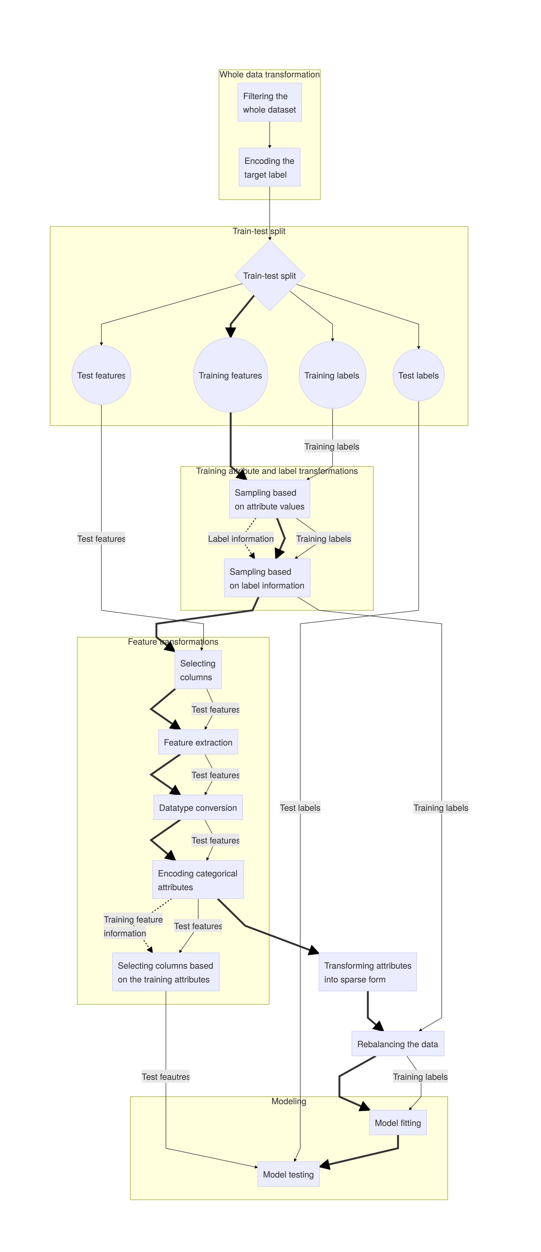
Appendix 1 - Data transformation steps <
Describing the steps of the workflow
1. Filtering the whole dataset
That in what degree we like to do this really depends on the actual problem we want to solve and also leads to the question of who, in what context, and with what kind of available data will try to predict the group responsible for the incident.
2. Encoding the target label
We need to do this early on because the codes need to be consistent between the training and test labels and neither we can transport the codes from one to the other because they do not share all their values with each other.
- We need to store the encoder model
- Sometimes 'Unknown' value codes need to be stored before the transformation
3. Train-test split
4. Training set
4.1. Sampling based on attribute values
This simply means that we train our model on only a subset of examples based on their values:
- If a subset of samples mirror 'better' the future instances, relying only on it might produce a better model. We can also give more weight to the important attributes. For the GTD, using only data from the last round of data collection (e.g. from the year 2015) might create better predictions because they represent better data collection methods. This is the same logic behind feature selection and extraction. However, when we do this based on actual values (e.g. year period, location, etc.) we change the number of samples (as opposed to column-wise transformations).
Because this tranformation changes sample size, we need to apply it also on the training labels.
4.2. Selecting columns
This is more straightforward than the previous case because the lack of columns does not effect the y labels although we might want to reindex the test samples for performance purposes.
4.3. Selecting samples based on label information
This is more tricky than the previous sample selection.
- Focusing only on groups responsible for more than one incident might be a viable option to emphasize their weight. On the other hand, we should not take them out from the test data because 'in real life' we cannot know whether the next one will be a one-off incident or not.
- Similarly, taking out the unknown groups might help the model to recognise groups in cross-validation but we definitely should not leave it out from the test set.
These transformations require
- information about the labels (frequency, the 'unknown' label), and
- applying the transformation also on the training labels (or doing there first, and applying on train_X).
4.4. Feature extraction
In this context this is basically the same category as simple feature selection. I does not influence the labels, but we need to apply this also on the test attributes.
4.5. Datatype conversion
This affects neither the labels nor the training data (if done well).
4.6. Encoding categorical attributes
This does not affect the labels but we need
- to apply this also on the test data, and
- optionally (e.g. for performance reasons), to select from the test data only those columns (now also representing actual values) which are in the training set.
4.7. Transforming attributes into sparse form
This can help us to use different algorithms. In our case, without it we could not be able to run SMOTE because, by default, it eats up all the memory on a standard Kaglle notebook.
4.8. Rebalancing the data
This both requires and transforms both the training attributes and labels, but should not affect test data.
5. Training labels
A summary of the already mentioned train_y transformations
- Sampling based on X_train attribute values
- Selecting samples based on label information
- Rebalancing together with X
6. Test set
While we have mentiond the necessary steps, I also summarize them here:
6.1. Test attributes
- Selecting columns (requires information form X_train)
- Feature extracion
- Datatype conversion
- Encoding categoricals
- Filtering on the training attributes (requires information from X_train) and transforming NaN values into zeros
6.2 Test labels
We do not need to do anything with the test_y, only after the test we might inverse recode it with the coder we used on the whole dataset at the start.
The image below shows an outline of the tranformations as I understood them at a particular time. I marked train_X transformations with bold because of their relatively central role in the workflow.