Lesson 2 - Image Classification Models from Scratch
#Run once per session
!pip install fastai -q --upgrade
Grab our vision related libraries
from fastai.vision.all import *
And our data
path = untar_data(URLs.MNIST)
Working with the data
items = get_image_files(path)
items[0]
PosixPath('/root/.fastai/data/mnist_png/training/0/12497.png')
Create an image object. Done automatically with ImageBlock.
im = PILImageBW.create(items[0])
im.show()
<matplotlib.axes._subplots.AxesSubplot at 0x7f104f532208>

Split our data with GrandparentSplitter, which will make use of a train and valid folder.
splits = GrandparentSplitter(train_name='training', valid_name='testing')
items[:3]
(#3) [/root/.fastai/data/mnist_png/training/0/12497.png,/root/.fastai/data/mnist_png/training/0/5475.png,/root/.fastai/data/mnist_png/training/0/33023.png]
Splits need to be applied to some items
splits = splits(items)
splits[0][:5], splits[1][:5]
([0, 1, 2, 3, 4], [60000, 60001, 60002, 60003, 60004])
Make a
DatasetsExpects items, transforms for describing our problem, and a splitting method
dsrc = Datasets(items, tfms=[[PILImageBW.create], [parent_label, Categorize]],
                  splits=splits)
We can look at an item in our Datasets with show_at
show_at(dsrc.train, 3)
<matplotlib.axes._subplots.AxesSubplot at 0x7f104ee21278>

We can see that it's a PILImage of a zero, along with a label of 0
Next we need to give ourselves some transforms on the data! These will need to:
- Ensure our images are all the same size
- Make sure our output are the
tensorour models are wanting - Give some image augmentation
tfms = [ToTensor(), CropPad(size=34, pad_mode=PadMode.Zeros), RandomCrop(size=28)]
ToTensor: Converts to tensorCropPadandRandomCrop: Resizing transforms- Applied on the
CPUviaafter_item
gpu_tfms = [IntToFloatTensor(), Normalize()]
- ``: Enables GPU usage
IntToFloatTensor: Converts to a floatNormalize: Normalizes data
dls = dsrc.dataloaders(bs=128, after_item=tfms, after_batch=gpu_tfms)
And show a batch
dls.show_batch()

From here we need to see what our model will expect
xb, yb = dls.one_batch()
And now the shapes:
xb.shape, yb.shape
(torch.Size([128, 1, 28, 28]), torch.Size([128]))
dls.c
10
So our input shape will be a [128 x 1 x 28 x 28] and our output shape will be a [128] tensor that we need to condense into 10 classes
The Model
Our models are made up of layers, and each layer represents a matrix multiplication to end up with our final y. For this image problem, we will use a Convolutional layer, a Batch Normalization layer, an Activation Function, and a Flattening layer
Convolutional Layer
These are always the first layer in our network. I will be borrowing an analogy from here by Adit Deshpande.
Our example Convolutional layer will be 5x5x1
Imagine a flashlight that is shining over the top left of an image, which covers a 5x5 section of pixels at one given moment. This flashlight then slides crosses our pixels at all areas in the picture. This flashlight is called a filter, which can also be called a neuron or kernel. The region it is currently looking over is called a receptive field. This filter is also an array of numbers called weights (or parameters). The depth of this filter must be the same as the depth of our input. In our case it is 1 (in a color image this is 3). Now once this filter begins moving (or convolving) around the image, it is multiplying the values inside this filter with the original pixel value of our image (also called element wise multiplications). These are then summed up (in our case this is just one multiplication of 28x28) to an individual value, which is a representation of just the top left of our image. Now repeat this until every unique location has a number and we will get what is called an activation or feature map. This feature map will be 784 different locations, which turns into a 28x28 array
def conv(ni, nf): return nn.Conv2d(ni, nf, kernel_size=3, stride=2, padding=1)
Here we can see our ni is equivalent to the depth of the filter, and nf is equivalent to how many filters we will be using. (Fun fact this always has to be divisible by the size of our image).
Batch Normalization
As we send our tensors through our model, it is important to normalize our data throughout the network. Doing so can allow for a much larger improvement in training speed, along with allowing each layer to learn independantly (as each layer is then re-normalized according to it's outputs)
def bn(nf): return nn.BatchNorm2d(nf)
nf will be the same as the filter output from our previous convolutional layer
Activation functions
They give our models non-linearity and work with the weights we mentioned earlier along with a bias through a process called back-propagation. These allow our models to learn and perform more complex tasks because they can choose to fire or activate one of those neurons mentioned earlier. On a simple sense, let's look at the ReLU activation function. It operates by turning any negative values to zero, as visualized below:
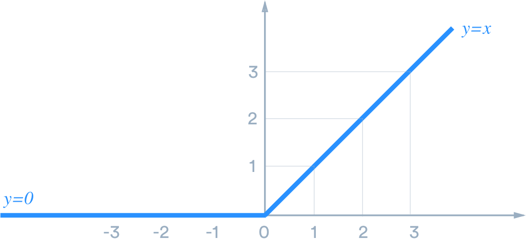
From "A Practical Guide to ReLU by Danqing Liu URL.
def ReLU(): return nn.ReLU(inplace=False)
Flattening
The last bit we need to do is take all these activations and this outcoming matrix and flatten it into a single dimention of predictions. We do this with a Flatten() module
Flatten??
Making a Model
- Five convolutional layers
nn.Sequential- 1 -> 32 -> 10
model = nn.Sequential(
    conv(1, 8),
    bn(8),
    ReLU(),
    conv(8, 16),
    bn(16),
    ReLU(),
    conv(16,32),
    bn(32),
    ReLU(),
    conv(32, 16),
    bn(16),
    ReLU(),
    conv(16, 10),
    bn(10),
    Flatten()
)
Now let's make our Learner
learn = Learner(dls, model, loss_func=CrossEntropyLossFlat(), metrics=accuracy)
We can then also call learn.summary to take a look at all the sizes with thier exact output shapes
learn.summary()
Sequential (Input shape: 128 x 1 x 28 x 28)
================================================================
Layer (type)         Output Shape         Param #    Trainable
================================================================
Conv2d               128 x 8 x 14 x 14    80         True
________________________________________________________________
BatchNorm2d          128 x 8 x 14 x 14    16         True
________________________________________________________________
ReLU                 128 x 8 x 14 x 14    0          False
________________________________________________________________
Conv2d               128 x 16 x 7 x 7     1,168      True
________________________________________________________________
BatchNorm2d          128 x 16 x 7 x 7     32         True
________________________________________________________________
ReLU                 128 x 16 x 7 x 7     0          False
________________________________________________________________
Conv2d               128 x 32 x 4 x 4     4,640      True
________________________________________________________________
BatchNorm2d          128 x 32 x 4 x 4     64         True
________________________________________________________________
ReLU                 128 x 32 x 4 x 4     0          False
________________________________________________________________
Conv2d               128 x 16 x 2 x 2     4,624      True
________________________________________________________________
BatchNorm2d          128 x 16 x 2 x 2     32         True
________________________________________________________________
ReLU                 128 x 16 x 2 x 2     0          False
________________________________________________________________
Conv2d               128 x 10 x 1 x 1     1,450      True
________________________________________________________________
BatchNorm2d          128 x 10 x 1 x 1     20         True
________________________________________________________________
Flatten              128 x 10             0          False
________________________________________________________________

Total params: 12,126
Total trainable params: 12,126
Total non-trainable params: 0

Optimizer used: <function Adam at 0x7f1070947a60>
Loss function: FlattenedLoss of CrossEntropyLoss()

Callbacks:
  - TrainEvalCallback
  - Recorder
  - ProgressCallback
learn.summary also tells us:
- Total parameters
- Trainable parameters
- Optimizer
- Loss function
- Applied
Callbacks
learn.lr_find()

Let's use a learning rate around 1e-1 (0.1)
learn.fit_one_cycle(3, lr_max=1e-1)
| epoch | train_loss | valid_loss | accuracy | time |
|---|---|---|---|---|
| 0 | 0.209175 | 0.159102 | 0.951200 | 01:14 |
| 1 | 0.123667 | 0.066494 | 0.978500 | 01:14 |
| 2 | 0.066589 | 0.038887 | 0.988300 | 01:14 |
Simplify it
- Try to make it more like
ResNet. ConvLayercontains aConv2d,BatchNorm2d, and an activation function
def conv2(ni, nf): return ConvLayer(ni, nf, stride=2)
And make a new model
net = nn.Sequential(
    conv2(1,8),
    conv2(8,16),
    conv2(16,32),
    conv2(32,16),
    conv2(16,10),
    Flatten()
)
Great! That looks much better to read! Let's make sure we get (roughly) the same results with it.
learn = Learner(dls, net, loss_func=CrossEntropyLossFlat(), metrics=accuracy)
learn.fit_one_cycle(3, lr_max=1e-1)
| epoch | train_loss | valid_loss | accuracy | time |
|---|---|---|---|---|
| 0 | 0.220734 | 0.197168 | 0.933900 | 01:15 |
| 1 | 0.130333 | 0.075714 | 0.975800 | 01:14 |
| 2 | 0.078764 | 0.041104 | 0.987000 | 01:15 |
Almost the exact same! Perfect! Now let's get a bit more advanced
ResNet (kinda)
The ResNet architecture is built with what are known as ResBlocks. Each of these blocks consist of two ConvLayers that we made before, where the number of filters do not change. Let's generate these layers.
class ResBlock(Module):
  def __init__(self, nf):
    self.conv1 = ConvLayer(nf, nf)
    self.conv2 = ConvLayer(nf, nf)

  def forward(self, x): return x + self.conv2(self.conv1(x))
- Class notation
__init__foward
Let's add these in between each of our conv2 layers of that last model.
net = nn.Sequential(
    conv2(1,8),
    ResBlock(8),
    conv2(8,16),
    ResBlock(16),
    conv2(16,32),
    ResBlock(32),
    conv2(32,16),
    ResBlock(16),
    conv2(16,10),
    Flatten()
)
net
Sequential(
  (0): ConvLayer(
    (0): Conv2d(1, 8, kernel_size=(3, 3), stride=(2, 2), padding=(1, 1), bias=False)
    (1): BatchNorm2d(8, eps=1e-05, momentum=0.1, affine=True, track_running_stats=True)
    (2): ReLU()
  )
  (1): ResBlock(
    (conv1): ConvLayer(
      (0): Conv2d(8, 8, kernel_size=(3, 3), stride=(1, 1), padding=(1, 1), bias=False)
      (1): BatchNorm2d(8, eps=1e-05, momentum=0.1, affine=True, track_running_stats=True)
      (2): ReLU()
    )
    (conv2): ConvLayer(
      (0): Conv2d(8, 8, kernel_size=(3, 3), stride=(1, 1), padding=(1, 1), bias=False)
      (1): BatchNorm2d(8, eps=1e-05, momentum=0.1, affine=True, track_running_stats=True)
      (2): ReLU()
    )
  )
  (2): ConvLayer(
    (0): Conv2d(8, 16, kernel_size=(3, 3), stride=(2, 2), padding=(1, 1), bias=False)
    (1): BatchNorm2d(16, eps=1e-05, momentum=0.1, affine=True, track_running_stats=True)
    (2): ReLU()
  )
  (3): ResBlock(
    (conv1): ConvLayer(
      (0): Conv2d(16, 16, kernel_size=(3, 3), stride=(1, 1), padding=(1, 1), bias=False)
      (1): BatchNorm2d(16, eps=1e-05, momentum=0.1, affine=True, track_running_stats=True)
      (2): ReLU()
    )
    (conv2): ConvLayer(
      (0): Conv2d(16, 16, kernel_size=(3, 3), stride=(1, 1), padding=(1, 1), bias=False)
      (1): BatchNorm2d(16, eps=1e-05, momentum=0.1, affine=True, track_running_stats=True)
      (2): ReLU()
    )
  )
  (4): ConvLayer(
    (0): Conv2d(16, 32, kernel_size=(3, 3), stride=(2, 2), padding=(1, 1), bias=False)
    (1): BatchNorm2d(32, eps=1e-05, momentum=0.1, affine=True, track_running_stats=True)
    (2): ReLU()
  )
  (5): ResBlock(
    (conv1): ConvLayer(
      (0): Conv2d(32, 32, kernel_size=(3, 3), stride=(1, 1), padding=(1, 1), bias=False)
      (1): BatchNorm2d(32, eps=1e-05, momentum=0.1, affine=True, track_running_stats=True)
      (2): ReLU()
    )
    (conv2): ConvLayer(
      (0): Conv2d(32, 32, kernel_size=(3, 3), stride=(1, 1), padding=(1, 1), bias=False)
      (1): BatchNorm2d(32, eps=1e-05, momentum=0.1, affine=True, track_running_stats=True)
      (2): ReLU()
    )
  )
  (6): ConvLayer(
    (0): Conv2d(32, 16, kernel_size=(3, 3), stride=(2, 2), padding=(1, 1), bias=False)
    (1): BatchNorm2d(16, eps=1e-05, momentum=0.1, affine=True, track_running_stats=True)
    (2): ReLU()
  )
  (7): ResBlock(
    (conv1): ConvLayer(
      (0): Conv2d(16, 16, kernel_size=(3, 3), stride=(1, 1), padding=(1, 1), bias=False)
      (1): BatchNorm2d(16, eps=1e-05, momentum=0.1, affine=True, track_running_stats=True)
      (2): ReLU()
    )
    (conv2): ConvLayer(
      (0): Conv2d(16, 16, kernel_size=(3, 3), stride=(1, 1), padding=(1, 1), bias=False)
      (1): BatchNorm2d(16, eps=1e-05, momentum=0.1, affine=True, track_running_stats=True)
      (2): ReLU()
    )
  )
  (8): ConvLayer(
    (0): Conv2d(16, 10, kernel_size=(3, 3), stride=(2, 2), padding=(1, 1), bias=False)
    (1): BatchNorm2d(10, eps=1e-05, momentum=0.1, affine=True, track_running_stats=True)
    (2): ReLU()
  )
  (9): Flatten()
)
Awesome! We're building a pretty substantial model here. Let's try to make it even simpler. We know we call a convolutional layer before each ResBlock and they all have the same filters, so let's make that layer!
def conv_and_res(ni, nf): return nn.Sequential(conv2(ni, nf), ResBlock(nf))
net = nn.Sequential(
    conv_and_res(1,8),
    conv_and_res(8,16),
    conv_and_res(16,32),
    conv_and_res(32,16),
    conv2(16,10),
    Flatten()
)
And now we have something that resembles a ResNet! Let's see how it performs
learn = Learner(dls, net, loss_func=CrossEntropyLossFlat(), metrics=accuracy)
learn.lr_find()

Let's do 1e-1 again
learn.fit_one_cycle(3, lr_max=1e-1)
| epoch | train_loss | valid_loss | accuracy | time |
|---|---|---|---|---|
| 0 | 0.156825 | 0.904546 | 0.756200 | 01:16 |
| 1 | 0.089813 | 0.063087 | 0.980300 | 01:16 |
| 2 | 0.040906 | 0.025675 | 0.992200 | 01:18 |