Universidade Federal do Rio Grande do Sul (UFRGS)
Programa de Pós-Graduação em Engenharia Civil (PPGEC)
PEC00144: Experimental Methods in Civil Engineering
Part II: Instrumentation
9. Review on electrical circuits
9.1. Voltage dividers and impedance
9.2. Power sources and batteries
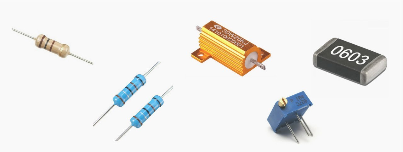
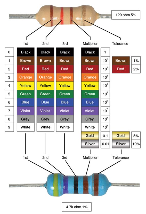
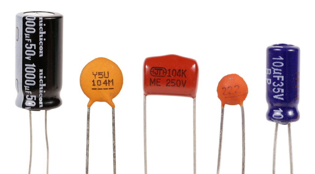
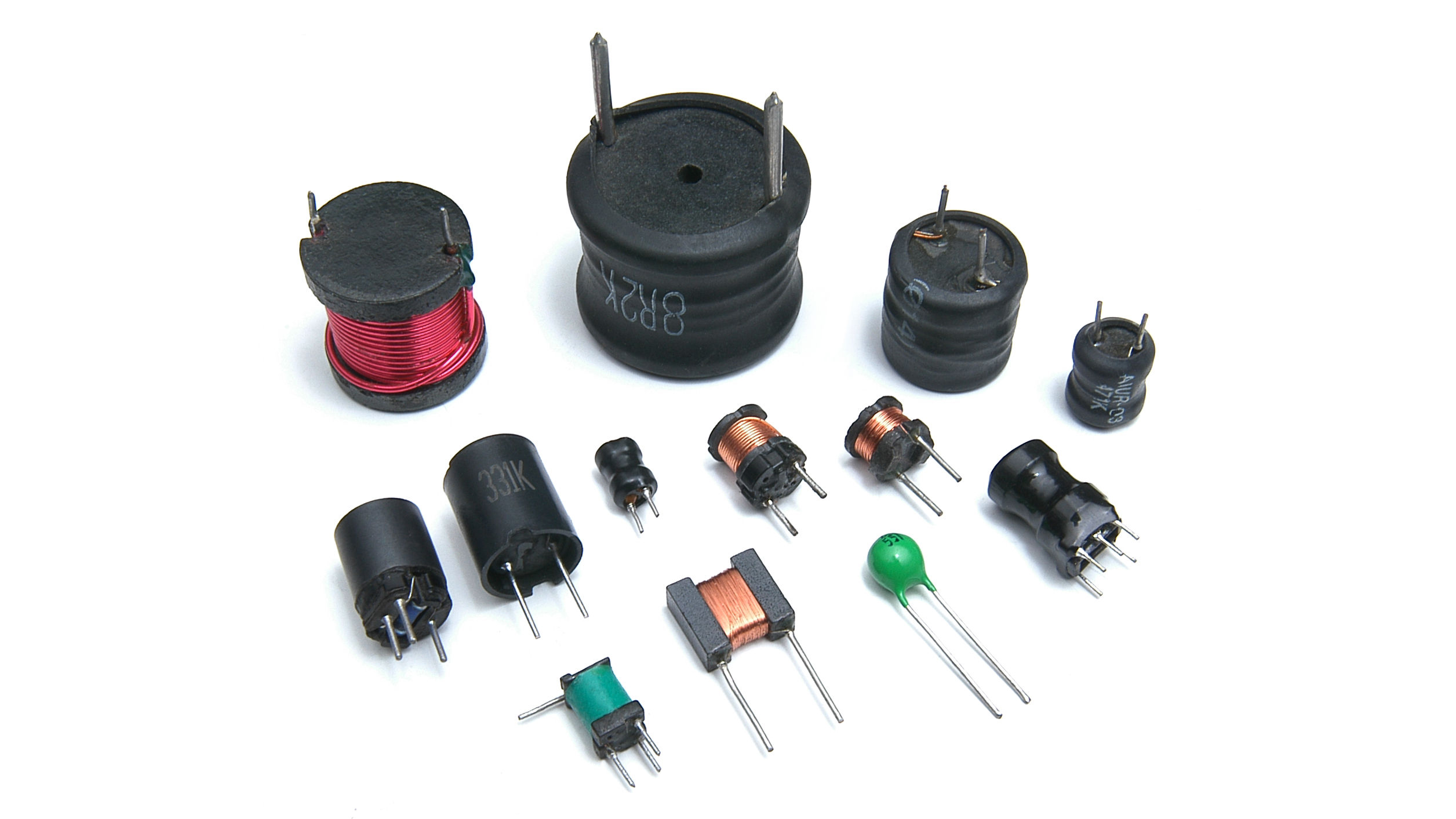
9.3. Passive circuit components
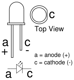
9.4. How to light up a LED
9.5. Low and high pass RC filters
9.6. Regulated voltage and current sources
9.7. Microprocessed power sources
Prof. Marcelo M. Rocha, Dr.techn. (ORCID)
Porto Alegre, RS, Brazil
# Importing Python modules required for this notebook
# (this cell must be executed with "shift+enter" before any other Python cell)

import numpy as np
import pandas as pd
import matplotlib.pyplot as plt
from   MRPy import MRPy
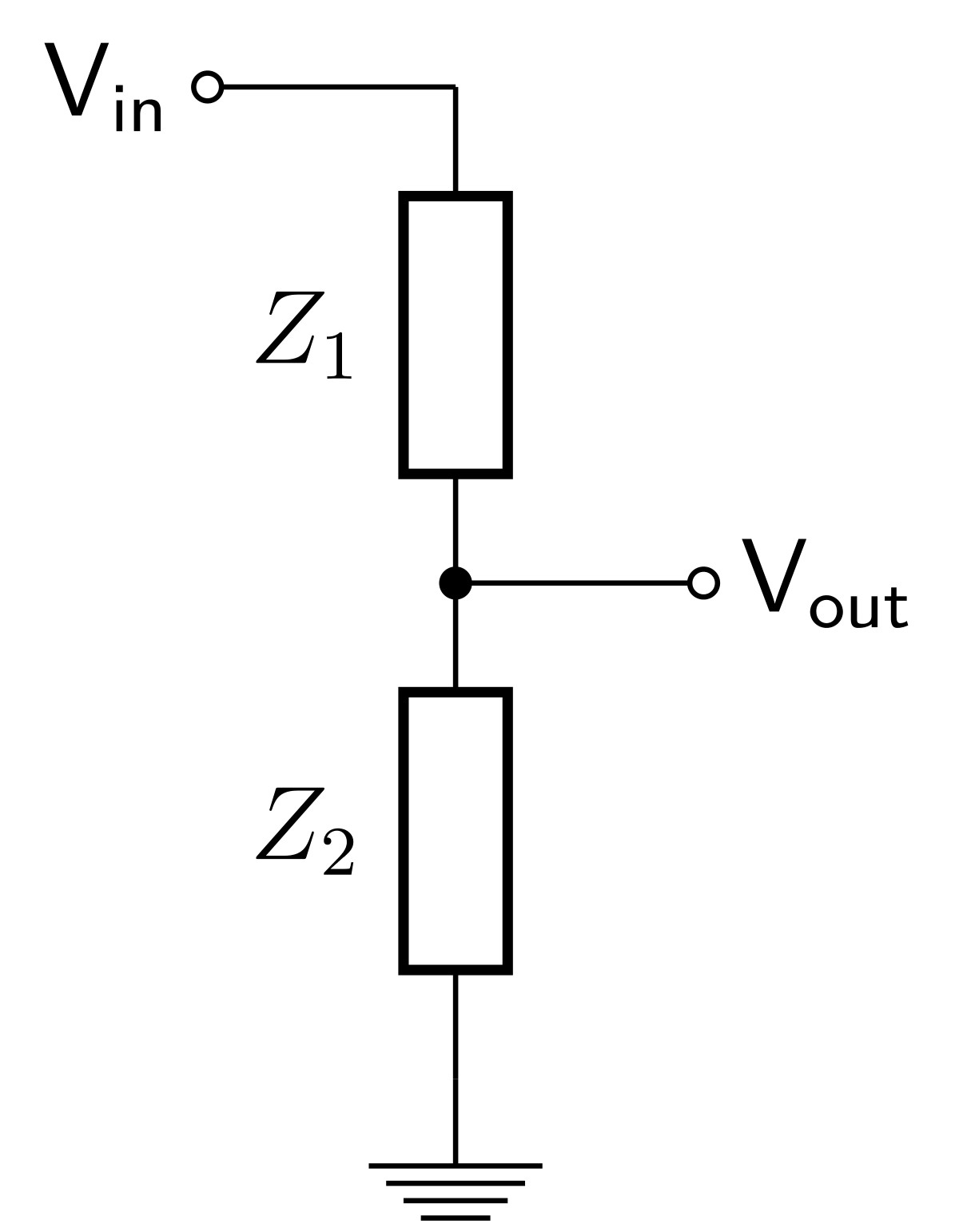
Vin  = 5.                # logic level 5V
Z1   = 5000.             # top resistor (ohms)
Z2   = 10000.            # bottom resistor (ohms)
Vout = Vin*Z2/(Z1 + Z2)  # logic level ~3.3V

print('Logic level output: {0:5.2f}V'.format(Vout))
Logic level output: 3.33V


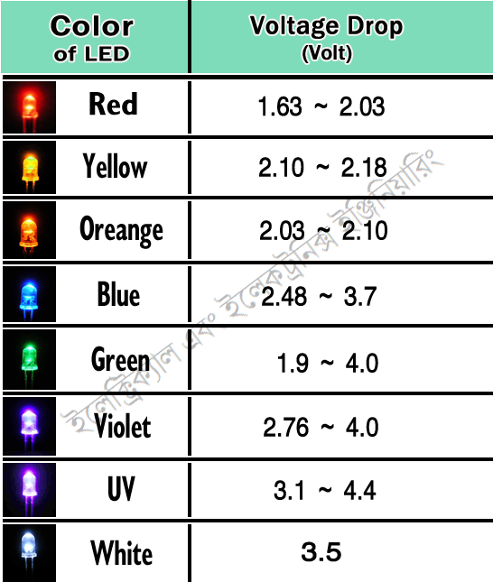
V_resist = 9000 - 1800      # voltage after a RED resistor (mV)
I_light  = 15.              # light up current (mA)

R = V_resist/I_light        # required resistor value (ohm)

print('Required resistor value: {0:5.1f}Ω'.format(R))
Required resistor value: 480.0Ω
9.5. Low and high pass RC filters 
For both low and high pass first order passive filters, with an association of a resistor and a capacitor, the cut off frequency is given by:
$$ f_{\rm 3dB} = \frac{1}{2\pi RC} $$The decibel is a measure of logarithmic relation to a reference value:
$$ {\rm dB} = 20 \log_{10} \left( \frac{V}{V_{\rm ref}} \right) $$Some important dB values:
| dB | ~fraction |
|---|---|
| −20 | 0.100 |
| −10 | 0.316 |
| −6 | 0.501 |
| −3 | 0.708 |
| +3 | 1.41 |
| +6 | 2.00 |
| +10 | 3.16 |
| +20 | 10. |
e1 =  0.;  f1 = 10.**e1           #  frequency domain
e2 =  4.;  f2 = 10.**e2

N  =  1000
f  =  np.logspace(e1, e2, N)
w  =  2*np.pi*f

C  =  0.1e-6                      #  100 nano Faraday
R  =  10.e03                      #  10 kilo Ohm
ZC = -1j/(w*C)

f3dB =  1/(2*np.pi*R*C);          # -3dB frequency

print('Cut off frequency (-3dB): {0:7.2f}Hz'.format(f3dB))
Cut off frequency (-3dB): 159.15Hz
9.5.1 Low pass

HLP   =  ZC/(R + ZC);
GLP   =  np.absolute(HLP);
dLP   =  20*np.log10(GLP);
pLP   =  180*np.angle(HLP)/np.pi;

fig1  =  plt.figure(1, figsize=(12,4));

sp11  =  plt.subplot(1,3,1)
sp11  =  plt.loglog(f,GLP);
sp11a =  plt.loglog([f3dB, f3dB], [0.1, 2], 'r', lw=2)
plt.title('Filter gain')
plt.axis([f1, f2, 0.1, 2]);
plt.grid(True);

sp12  =  plt.subplot(1,3,2)
sp12  =  plt.semilogx(f,dLP);
sp12a =  plt.semilogx([f3dB, f3dB], [-20, 5], 'r', lw=2)
plt.title('Filter gain in dB')
plt.axis([f1, f2, -20, 5]);
plt.grid(True);

sp13  =  plt.subplot(1,3,3)
sp13  =  plt.semilogx(f,pLP);
sp13a =  plt.semilogx([f3dB, f3dB], [-120, 30], 'r', lw=2)
plt.title('Filter phase shift')
plt.axis([f1, f2, -120, 30]);
plt.grid(True);

9.5.2 High pass
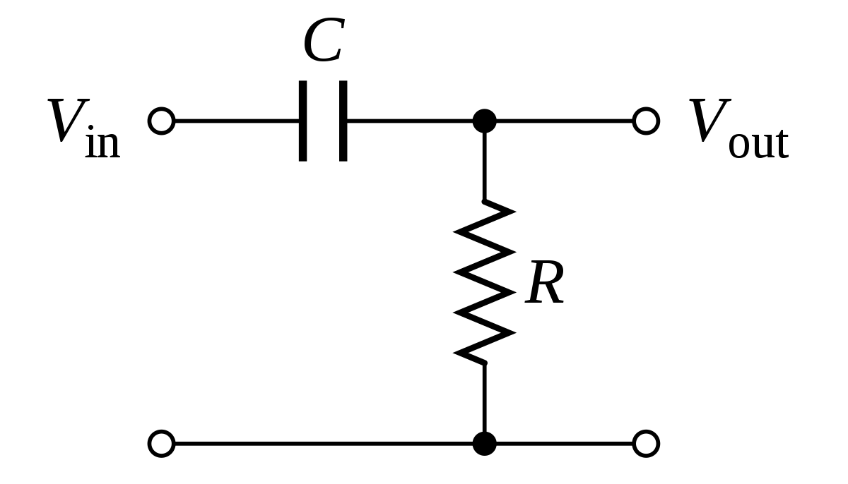
HHP   =  R/(R + ZC);
GHP   =  np.absolute(HHP);
dHP   =  20*np.log10(GHP);
pHP   =  180*np.angle(HHP)/np.pi;

fig1  =  plt.figure(1, figsize=(12,4));

sp11  =  plt.subplot(1,3,1)
sp11  =  plt.loglog(f,GHP);
sp11a =  plt.loglog([f3dB, f3dB], [0.1, 2], 'r', lw=2)
plt.title('Filter gain')
plt.axis([f1, f2, 0.1, 2]);
plt.grid(True);

sp12  =  plt.subplot(1,3,2)
sp12  =  plt.semilogx(f,dHP);
sp12a =  plt.semilogx([f3dB, f3dB], [-20, 5], 'r', lw=2)
plt.title('Filter gain in dB')
plt.axis([f1, f2, -20, 5]);
plt.grid(True);

sp13  =  plt.subplot(1,3,3)
sp13  =  plt.semilogx(f,pHP);
sp13a =  plt.semilogx([f3dB, f3dB], [-30, 120], 'r', lw=2)
plt.title('Filter phase shift')
plt.axis([f1, f2, -30, 120]);
plt.grid(True);

Example of application: the low pass filtering capacitor for MEMS accelerometer ADXL203, with an output resistor of 32kΩ.
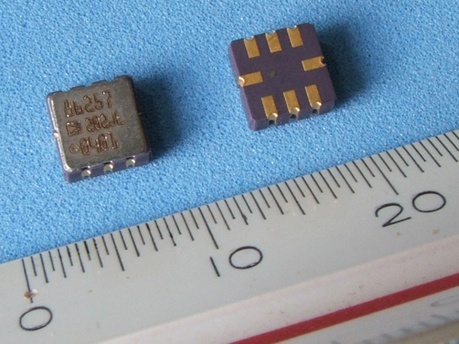
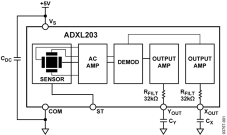
f3dB = 50.         # set -3dB cut off frequency
R    = 32000.      # internal output resistance

C    = 1/(2*np.pi*R*f3dB)

print('Minimum capacitor value: {0:7.2f}muF'.format(1e6*C))
Minimum capacitor value: 0.10muF
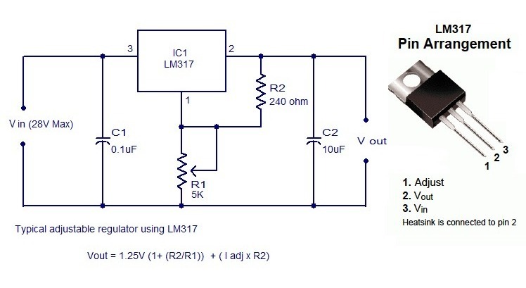
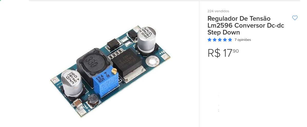
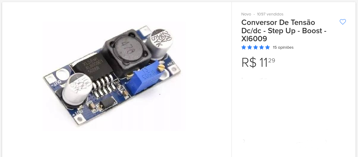
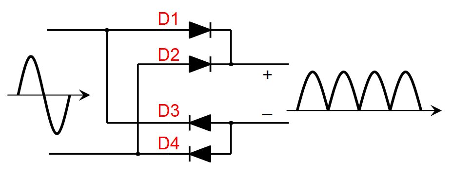
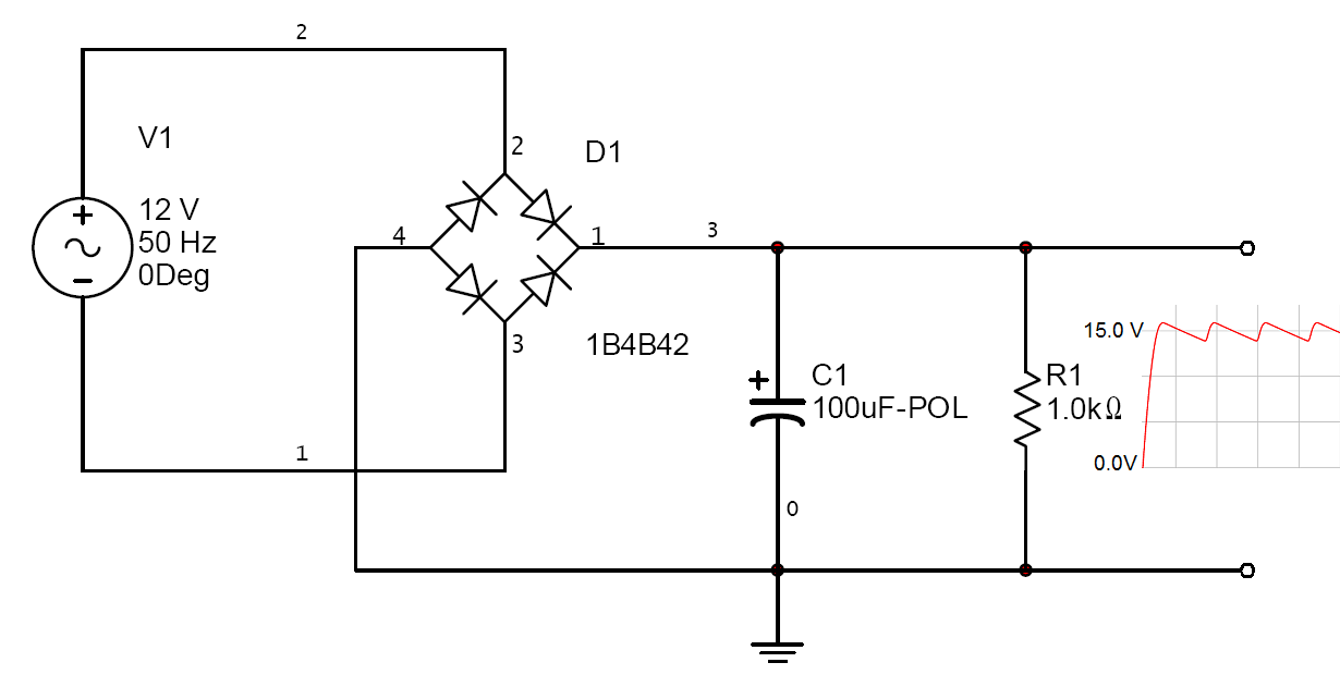
9.6. Regulated voltage and current sources 
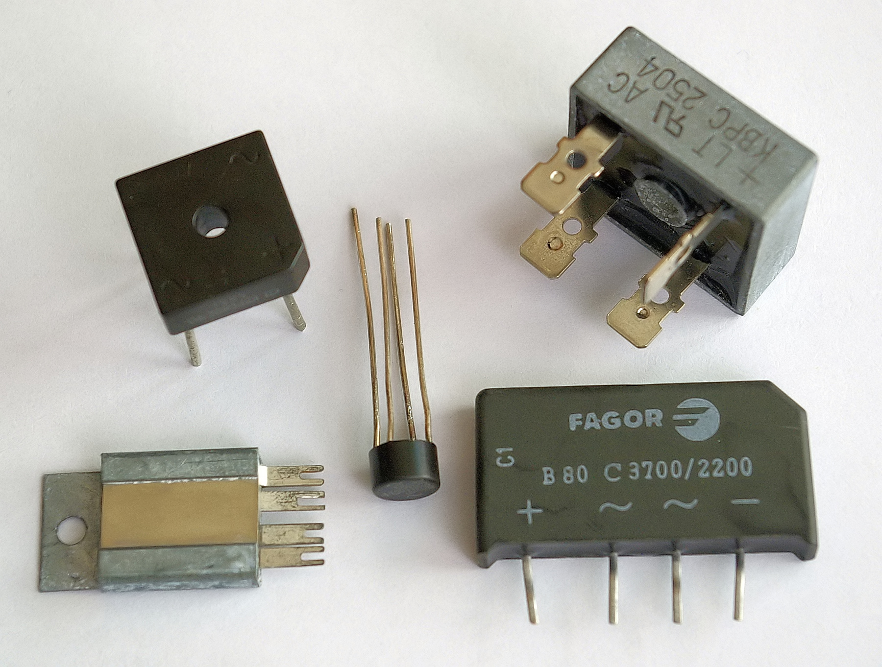
AC to DC conversion with diode bridges:
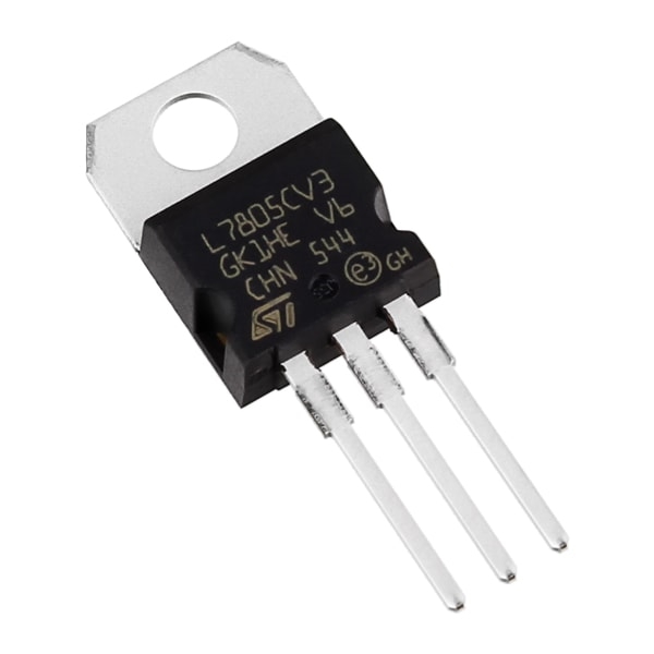
Fixed voltage regulator:
Variable voltage regulator: