Universidade Federal do Rio Grande do Sul (UFRGS)
Programa de Pós-Graduação em Engenharia Civil (PPGEC)
PEC00144: Experimental Methods in Civil Engineering
Part II: Instrumentation
8.1. Autocovariance function and stationarity
8.2. Fourier series and Fourier transform
8.3. Power spectral density and periodograms
8.4. White noise and pink noise
8.5. Signal derivation and integration
8.6. Basic stationarity test
8.7. Level upcrossing rate and peak factor
8.8. Frequency domain signal filtering
8.9. Cross correlation and coherence functions
Prof. Marcelo M. Rocha, Dr.techn. (ORCID)
Porto Alegre, RS, Brazil
# Importing Python modules required for this notebook
# (this cell must be executed with "shift+enter" before any other Python cell)

import numpy as np
import pandas as pd
import matplotlib.pyplot as plt

from   MRPy import MRPy
8. Analog signals processing 
8.1. Autocovariance function and stationarity 
Analog signals are the outcome of some physical measurement, usually some electrical quantity like voltage, current, or electric charge. The magnitude of such quantities are expected to be analogous to some observed physical quantity, like stress, force, displacement, acceleration, etc.
An analog signal is generally considered as a random process, $X(t)$. A random process is a time dependent random variable, what requires its statistical properties to be also regarded as time dependent.
The autocovariance function, $C_X(\tau)$, of a random process, $X(t)$, is defined as the first cross moment between the process amplitude at two time instants:
$$ C_X(t_1, t_2) = {\rm E}\left\{ X(t_1) X(t_2) \right\} - \mu_1\mu_2$$where $\mu_1$ and $\mu_2$ are the mean value of $X(t)$ at instants $t_1$ and $t_2$, respectively. If a random process is stationary, its statistical properties are assumed to be independent of time, and the expression above depends only on the time gap, $\tau = t_2 - t_1$:
$$ C_X(\tau) = {\rm E}\left\{ X(t) X(t + \tau) \right\} - \mu_X^2 $$The definitions above exclude the mean value of $X(t)$, keeping only the time dependent part of its amplitude. Furthermore, it is evident that the autocovariance function is a pair function (symmetric over the axis $\tau = 0$) and that at origin:
$$ C_X(0) = {\rm E}\left\{ X^2(t) \right\} - \mu_X^2 = \sigma_X^2$$which is the process variance. The autocovariance function can be normalized by $\sigma_X^2$ resulting in the process autocorrelation function:
$$ R^2_X(\tau) = \frac{C_X(\tau)}{\sigma_X^2} $$which is also a pair function such that $-1 \leq R_X(\tau) \leq +1$.
8.2. Fourier series and Fourier transform 
An introduction to Fourier analysis can be found in Class 7 of the course Introduction to Vibration Theory.
8.3. Power spectral density and periodograms 
The power spectral density, $S_X(\omega)$, of a stationary random process is defined as the Fourier transform of the autocovariance function, $C_X(\tau)$:
$$ S_X(\omega) = \frac{1}{2\pi} \int_{-\infty}^{+\infty} {C_X(\tau) e^{-i\omega\tau} \, d\tau}$$This means that $S_X(\omega)$ and $C_X(\tau)$ are a Fourier transform pair, and consequently:
$$ C_X(\tau) = \int_{-\infty}^{+\infty} {S_X(\omega) e^{i\omega\tau} \, d\omega} $$The definitions above implies that:
$$ C_X(0) = \int_{-\infty}^{+\infty} {S_X(\omega) \, d\omega} = \sigma_X^2$$what means that the total integral of the spectral density is, by definition, the process variance.
The MRPy module provides a straightforward method for visualizing the
spectral density estimator, called periodogram, and the corresponding autocorrelation
function. Below is a short script where a cosine wave is analysed:
Td   =  2.           # total signal duration (s)
fs   =  512          # sampling rate (Hz)
N    =  int(Td*fs)   # total number of samples

f0   =  8.           # cosine wave frequency (Hz)

X0   =  MRPy.harmonic(NX=1, N=N, fs=fs, X0=1.0, f0=f0, phi=0.0)

f00  =  X0.plot_time(fig=0, figsize=(8,3), axis_t=[0, Td, -2.0, 2.0])
f01  =  X0.plot_freq(fig=1, figsize=(8,3), axis_f=[0, 16,  0.0, 2.0])    # periodogram
f02  =  X0.plot_corr(fig=2, figsize=(8,3), axis_T=[0,  1, -2.0, 2.0])    # autocovariance


It can be seen that the periodogram of a sine signal is a impulse function at the sine frequency.
Below it is show how to simulate a process with given autocorrelation function.
Sx, fs =  X0.periodogram()
X1     =  MRPy.from_periodogram(Sx, fs)

f00    =  X1.plot_time(fig=0, figsize=(8,3), axis_t=[0, Td, -2.0, 2.0])
f01    =  X1.plot_freq(fig=1, figsize=(8,3), axis_f=[0, 16,  0.0, 2.0])    # periodogram
f02    =  X1.plot_corr(fig=2, figsize=(8,3), axis_T=[0,  1, -2.0, 2.0])    # autocovariance

tau    =  X1.T_axis()
kt     = (tau <= 0.5)
Cx     =  np.zeros(tau.shape)
Cx[kt] =  1 - 2*tau[kt]

X2     =  MRPy.from_autocov(Cx, tau[-1])

f00    =  X2.plot_time(fig=0, figsize=(8,3), axis_t=[0, 8, -4.0,  4.0])
f01    =  X2.plot_freq(fig=1, figsize=(8,3), axis_f=[0, 8,  0.0,  2.0])
f02    =  X2.plot_corr(fig=2, figsize=(8,3), axis_T=[0, 4, -2.0,  2.0])


8.4. White noise and pink noise 
A Gaussian white noise is a signal with random amplitude with normal distribution and a constant power density all over the frequency domain:
$$ S_X(\omega) = S_0 $$The associated autocorrelation function is a Dirac's Delta at the origin, with an infinite pulse integral. This signal in practice must have a limited band, otherwise the corresponding variance would be infinite. For practical purposes a signal is considered to be a white noise if the power is constant (within some statistical error) over some relevant frequency band $\Delta\omega = \omega_2 - \omega_1$:
$$ S_X(\omega) = S_0, \hspace{5mm} {\rm for} \hspace{5mm} \omega_1 \leq \omega \leq \omega_2 $$and zero otherwise. The corresponding autocorrelation function is:
$$C_X(\tau) = \frac{4S_0}{\tau} \sin\left( \frac{ \Delta\omega}{2} \tau \right) \cos\left( \omega_0 \tau \right) $$where $\omega_0 = (\omega_1 + \omega_2)/2$ is the band center. The corresponding variance is:
$$ \sigma_X^2 = C_X(0) = 2\Delta\omega S_0$$As the band width $\Delta\omega$ decreases, the signal above approaches a cosine wave with frequency $\omega_0$, as described in the previous section.
Let us take a look on a band-limited Gaussian white noise simulation with MRPy.
The simulation uses $S_0 = 1$, hence the standard deviation will be
$\sigma_X = \sqrt{2\Delta\omega}$.
X = MRPy.white_noise(NX=1, N=2**15, fs=512, band=[1, 100])

print('Mean value:         {0:7.4f}'.format(X[0].mean()))
print('Standard deviation: {0:7.4f}'.format(X[0].std()),'\n')

f03 = X.plot_time(fig=3, figsize=(8,3), axis_t=[0, Td, -10.00, 10.00])
f04 = X.plot_freq(fig=4, figsize=(8,3), axis_f=[0, 32,   0.00,  1.00])
f05 = X.plot_corr(fig=5, figsize=(8,3), axis_T=[0,  1,  -1.00,  1.00])
Mean value:         -0.0000
Standard deviation:  1.0000


The MRPy module uses a simulation technique that gives an almost perfectly
constant periodogram, as specified.
8.5. Signal derivation and integration 
As a starting point, let us calculate the following derivative:
$$ \frac{d}{d\tau}\left[ X(t) X(t+\tau) \right] = X(t) \cdot \frac{d X(t + \tau)}{d(t+\tau)} \cdot \frac{d(t+\tau)}{dt} = X(t) \dot{X}(t+\tau) $$Now, using the expected value operator and considering autocovariance symmetry:
$$ \frac{d C_X(\tau)}{d\tau} = {\rm E}\left\{ X(t) \dot{X}(t+\tau) \right\} = {\rm E}\left\{ X(t-\tau) \dot{X}(t) \right\} $$and following the logic to find the second derivative:
$$ \frac{d^2 C_X(\tau)}{d\tau^2} = -{\rm E}\left\{\dot{X}(t) \dot{X}(t+\tau) \right\} = - C_{\dot{X}} (\tau)$$With this result at hand, we go back to the relation between power density and autocovariance:
$$ C_X(\tau) = \int_{-\infty}^{+\infty} {S_X(\omega) e^{i\omega\tau} \, d\omega} $$and apply double derivative:
\begin{align*} \frac{d C_X(\tau)}{d\tau} &= \int_{-\infty}^{+\infty} {i\omega S_X(\omega) e^{i\omega\tau} \, d\omega} \\ \frac{d^2 C_X(\tau)}{d\tau^2} &= - \int_{-\infty}^{+\infty} {\omega^2 S_X(\omega) e^{i\omega\tau} \, d\omega} \end{align*}Now, considering that the following relation is also valid:
$$ C_\dot{X}(\tau) = \int_{-\infty}^{+\infty} {S_\dot{X}(\omega) e^{i\omega\tau} \, d\omega} $$It finally results that:
\begin{align*} S_\dot{X} (\omega) &= \omega^2 S_{X} (\omega) \\ S_\ddot{X}(\omega) &= \omega^4 S_{X}(\omega) \end{align*}These relations allow us to calculate the spectral density of velocity and acceleration processes from the spectral density of displacement process, or vice-versa. They are quite useful for converting signal amplitudes obtained with one type of transducer (for instance, an accelerometer) to amplitudes as they would have been obtained with other type of transducer (for instance, displacement).
The MRPy class provides the calculation of derivatives and integrals in
frequency domain, as demonstrated below. The methods allow the definition
of a passing frequency band, for simultaneously eliminating noise errors.
acc =  MRPy.white_noise(N=2**15, fs=512) + 0.001*MRPy.harmonic(N=2**15, fs=512, f0=0.5)
Td  =  acc.Td

f03 =  acc.plot_time(fig=3, figsize=(8,3), axis_t=[0,  Td, -10.00, 10.00])
f04 =  acc.plot_freq(fig=4, figsize=(8,3), axis_f=[0,   1,   0.00,  0.01])
f05 =  acc.plot_corr(fig=5, figsize=(8,3), axis_T=[0, 0.1,  -1.00,  1.00])


V1  =  acc.integrate()               # integration without filtering
#V1  =  acc.differentiate()           # integration without filtering

f03 =  V1.plot_time(fig=3, figsize=(8,3))#, axis_t=[0,  Td, -0.50, 0.50])
f04 =  V1.plot_freq(fig=4, figsize=(8,3))#, axis_f=[0,  2,   0.00, 0.10])
f05 =  V1.plot_corr(fig=5, figsize=(8,3))#, axis_T=[0, 32,  -1.00, 1.00])


V2   =  acc.integrate(band=[0.3, 0.7])         # integration with filtering

f06  =  plt.figure(6, figsize=(8,3))
f06a =  plt.plot(V1.t_axis(), V1[0], 'r')
f06b =  plt.plot(V2.t_axis(), V2[0], 'b')

#plt.axis([0, Td, -1, 1])
plt.grid(True)

Whenever a signal is integrated without a low frequency cut, a zero drift is expected to happen! This can be avoided by setting a lower frequency bound as high as possible without attenuating the useful part of the signal.
8.6. Basic stationarity test 
Previously we have demonstrated that:
$$ \frac{d C_X(\tau)}{d\tau} = {\rm E}\left\{ X(t) \dot{X}(t+\tau) \right\} = \int_{-\infty}^{+\infty} {i\omega S_X(\omega) e^{i\omega\tau} \, d\omega} $$By making $\tau = 0$ in the relations above gives:
$$ {\rm E}\left\{ X(t) \dot{X}(t) \right\} = \int_{-\infty}^{+\infty} {i\omega S_X(\omega) \, d\omega} $$The power spectral density is a pair function. Multiplying it by $i\omega$ necessarily yields an odd function. Consequently the integral vanishes and:
$$ {\rm E}\left\{ X(t) \dot{X}(t) \right\} = 0 $$This relation can be a shortcut for ascertaining the signal stationarity and hence validating the constancy of its spectral density.
This result can be demonstrated through simulation with the MRPy module.
A Gaussian white noise is simulated and its derivative is calculated. Both
procedures restrain the signals to the same limited band:
X    =  MRPy.white_noise(NX=1, N=2**15, fs=512, band=[8, 16])
Xdot =  X.differentiate(band=[8, 16])

f07  =  plt.figure(7, figsize=(3,3))
f07a =  plt.plot(X[0], Xdot[0], 'b.')

#plt.axis([-10, 20, -500, 500])
plt.grid(True)

print(np.corrcoef(X, Xdot))
[[1.00000000e+00 2.98538788e-18]
 [2.98538788e-18 1.00000000e+00]]

The lack of correlation between the process and its derivative observed in the plot above is an evidence of process stationarity.
8.7. Level upcrossing and peak factors 
For a stationary process, the expected number of upcrossings, $N^{+}_a(T)$, of a given amplitude level, $a$, within a given observation time, $T$, is given by:
$$ N^{+}_a(T) = \nu^{+}_a T$$where $\nu^{+}_a$ is the upcrossing rate of level $a$. In other words, the number of upcrossings is proportional to the observation time.
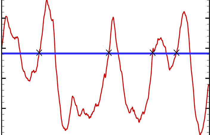
The upcrossing rate is calculated by integrating the joint probability distribution of the process amplitude and its derivative, such that the amplitude is fixed at level $a$ and only positive values are regarded for its derivative:
$$ \nu^{+}_a = \int_0^{\infty} {p_{X\dot{X}}(x=a, \dot{x}) \, x \, d{\dot{x}}} $$This result can be particularized for a Gaussian process, also considering that stationarity implies that the process and its derivative are uncorrelated:
$$ \nu^{+}_a = \frac{1}{2\pi} \, \frac{\sigma_\dot{X}}{\sigma_X} \, \exp \left( -\frac{a^2}{2\sigma_X^2} \right) $$Recalling from previous results that:
$$ \sigma_X^2 = \int_{-\infty}^{+\infty} {S_X(\omega) \, d\omega} $$and that:
$$ \sigma_\dot{X}^2 = \int_{-\infty}^{+\infty} {\omega^2 S_X(\omega) \, d\omega} $$allow us to estimate the upcrossing rate for any stationary signal by integrating the periodogram as indicated above.
Para a parcela flutuante da resposta em deslocamento, como a análise foi conduzida no domínio da frequência, resultados no domínio do tempo só pode ser obtidos em termos estatísticos. A abordagem da NBR-6123 consiste em se adotar um fator de pico da resposta modal $g_k = 4$, aplicado sobre o desvio padrão da resposta flutuante. No entanto, já que o espectro da resposta está disponível, é possível obter-se uma estimativa mais precisa deste fator de pico utilizando-se a fórmula de Davenport:
$$g_k = \sqrt{2 \ln (\nu^{+}_0 T)} + \frac{0.5772}{\sqrt{2 \ln (\nu^{+}_0 T)}}$$onde $T$ é o tempo de observação, adotado como 600s na NBR-6123, e $\nu_k$ é a taxa de cruzamento do nível zero para o positivo (zero upcrossing rate), calculada a partir do espectro como:
$$ \nu^{+}_0 = \sqrt{\frac{\int_0^\infty{f^2 S_X(f) \; df}} {\int_0^\infty{ S_X(f) \; df}}} $$Observe-se que o denominador dentro da raiz é a variância da resposta modal.
Aplicando-se as expressões acima ao exemplo de cálculo tem-se:
T   =  2000

X   =  MRPy.white_noise(N=2**16, Td=T)     # full band white noise
Y   =  X.sdof_Duhamel(4, 0.01)             # mass-spring system response
Y   =  Y/Y[0].std()                        # forces deviation equal to 1

Tm  =  X.Td
gD  =  Y.Davenport(T=T)                    # Gaussian narrow-band process
gS  =  Y.splitmax (T=T)                    # Prof. Rocha's method

Ypk = Y[0].mean() + gD[0]*Y[0].std()       # mean + g.deviation

print('Peak factor from Davenport:  {0:6.3f}'.format(gD[0]))
print('Peak factor from splitmax:   {0:6.3f}'.format(gS[0]))
print('Peak value for displacement: {0:6.3f}'.format(Ypk))

f09  =  plt.figure(9, figsize=(12,4))
f09a =  plt.plot(Y.t_axis(), Y[0], 'r', lw=1)

plt.axis([0, X.Td, -6, 6])
plt.grid(True)
Peak factor from Davenport:   4.376
Peak factor from splitmax:    3.944
Peak value for displacement:  4.377

Portanto, o pico do processo é dado por:
$$ {\rm E}\left\{ X_{\rm peak} \right\} = \mu_X + g_k \sigma_X $$8.8. Frequency domain signal filtering 
Td   =  4.           # total signal duration
fs   =  2048         # sampling rate
N    =  int(Td*fs)   # total number of samples
f60  =  60.          # sinus wave frequency

t    =  np.linspace(0, Td, N)
xi   =  np.sin(10*np.pi*t) + np.random.randn(N) + np.cos(2*np.pi*f60*t)
X    =  MRPy(xi, fs=fs)

Y    =  X.filtered(band=[0, 20], mode='pass') # try out also 'stop'

f08  =  plt.figure(8, figsize=(12,4))
f08a =  plt.plot(X.t_axis(), X[0], 'r', lw=0.5)
f08b =  plt.plot(Y.t_axis(), Y[0], 'b', lw=0.8)

plt.axis([0, 1, -10, 10])
plt.grid(True)

Y.plot_freq(fig=9, figsize=(12,4), axis_f=[0, 100, 0, 2])
[[<matplotlib.lines.Line2D at 0x1aea171aa40>]]
