Universidade Federal do Rio Grande do Sul (UFRGS)
Programa de Pós-Graduação em Engenharia Civil (PPGEC)
PEC00144: Experimental Methods in Civil Engineering
Part I: Analysis
2. Design of reduced scale models
2.1. Example: elastic beam under self weight
2.1.1. Model type "replica"
2.1.2. Model type "equivalent"
2.2. Example: cable catenary
2.3. Assignment
Prof. Marcelo M. Rocha, Dr.techn. (ORCID)
Porto Alegre, RS, Brazil
# Importing Python modules required for this notebook
# (this cell must be executed with "shift+enter" before any other Python cell)

import numpy as np
import pandas as pd
import matplotlib.pyplot as plt

# Importing pandas dataframe with dimension exponents for relevant quantities

DimData = pd.read_excel('resources/DimData.xlsx',
                         index_col  =  0,
                         header     =  0,
                         sheet_name = 'DimData')

DimData
| descriptor | latex | L | M | T | |
|---|---|---|---|---|---|
| a | Acceleration | a | 1 | 0 | -2 |
| α | Angular acceleration | \alpha | 0 | 0 | -2 |
| ω | Angular frequency | \omega | 0 | 0 | -1 |
| A | Area | A | 2 | 0 | 0 |
| EA | Axial stiffness | EA | 1 | 1 | -2 |
| EI | Beam bending stiffness | EI | 3 | 1 | -2 |
| GAs | Beam shear stiffness | GA_s | 1 | 1 | -2 |
| ρ | Density | \rho | -3 | 1 | 0 |
| μ | Dynamic viscosity | \mu | -1 | 1 | -1 |
| F | Force | F | 1 | 1 | -2 |
| q | Force per unit length | q | 0 | 1 | -2 |
| f | frequency | f | 0 | 0 | -1 |
| υ | Kinematic viscosity | \nu | 2 | 0 | -1 |
| L | Length | L | 1 | 0 | 0 |
| m | Mass | m | 0 | 1 | 0 |
| im | Mass inertia per unit length | i_m | 1 | 1 | 0 |
| μA | Mass per unit area | \mu_A | -2 | 1 | 0 |
| μL | Mass per unit length | \mu_L | -1 | 1 | 0 |
| M | Moment | M | 2 | 1 | -2 |
| I | Moment of inertia | I | 4 | 0 | 0 |
| W | Resistent modulus | W | 3 | 0 | 0 |
| Im | Rotational mass inertia | I_m | 2 | 1 | 0 |
| k | Spring stiffness | k | 0 | 1 | -2 |
| σ | Stress | \sigma | -1 | 1 | -2 |
| t | Time | t | 0 | 0 | 1 |
| v | Velocity | v | 1 | 0 | -1 |
| c | Viscous damping | c | 0 | 1 | -1 |
| V | Volume | V | 3 | 0 | 0 |
2. Design of reduced scale models 
2.1. Example: elastic beam under self-weight 
Let us design a reduced model for a reinforced concrete simply supported beam, as depicted below. The total span is $L = 10$m and other relevant quantities are:
- Rectangular cross section:
$B\times H = 0.2 \times 0.5{\rm m}$
Hence the section properties are:
$A = 0.1{\rm m}^2$ e $I = 0.002083 {\rm m}^4$ - Density of reinforced concrete:
$\rho = 2500 {\rm kg/m}^3$
Hence the mass per unit length is:
$\mu_L = \rho A = 2500 \times 0.1 = 250{\rm kg/m}$ - Young's modulus for concrete:
$E_{\rm c} = 30 \times 10^{9} {\rm N/m}^2$
Hence the flexural stiffness is:
$E_{\rm c}I = 62.5\times 10^6 {\rm Nm}^2$

We wish to measure the maximum displacement at beam center, $w_{\rm max}$ caused by self weight. The theoretical formula for this displacement is:
$$ w_{\rm max} = \frac{5}{384} \frac{q L^4}{EI} $$wherer $q = \mu_L g$, with $g \approx 9.81{m/s^2}$. Replacing values gives:
B  = 0.2
H  = 0.5
L  = 10.
ρ  = 2500.
g  = 9.81
E  = 3.e10

A  = B*H
I  = B*(H**3)/12
EI = E*I
μL = ρ*A
q  = μL*g

w_max = (5/384)*q*(L**4)/EI

print('Theoretical displacement at beam center is {0:5.2f}mm'.format(1000*w_max))
Theoretical displacement at beam center is 5.11mm
The theoretical formula indicates that the governing quantities are the mass per unit length (or the distributed load) and the flexural stiffness.
2.1.1. Model type "replica" 
Let us now design a reduced scale model. The length scale is chosen as 1m:10m, while the acceleration scale must be assumed to be 1g:1g, for the model will be tested under the same gravity. Let us further assume that our model will be built with aluminum, what implies that the Young's modulus has as a 71GPa:30GPa scale, which is the same as the stress scale.
The resulting new base is then:
ABC    = ['L', 'a', 'σ']           # selected quantities for the new base
LMT    = ['L', 'M', 'T']           # dimensions are the last 3 columns of DimData
base   =  DimData.loc[ABC, LMT]    # the dimensional matrix
i_base =  np.linalg.inv(base)      # base inversion

base
| L | M | T | |
|---|---|---|---|
| L | 1 | 0 | 0 |
| a | 1 | 0 | -2 |
| σ | -1 | 1 | -2 |
The scales for the quantities adopted for the new base are:
λ_L    =  1/10         # length scale for the reduced model
λ_a    =  1/1          # acceleration remains unchanged (same gravity)
λ_σ    = 71/30         # model built with aluminum instead of concrete
Now we calculate the scales for further quantities that are relevant to build the reduced model and interpreting results. They could be force, $F$, distributed load, $q$, the beam cross section flexural stiffness, $EI$, and the mass per unit length, $\mu_L$. The calculations are carried out as explained in Class 2. Firstly we prepare the dimensional matrix for the selected quantities:
par    = ['F', 'q', 'EI', 'μL', 'ρ']         # selected scales to be calculated
npar   =  len(par)                           # number of quantities
DimMat =  DimData.loc[par, LMT]              # the dimensional matrix

DimMat
| L | M | T | |
|---|---|---|---|
| F | 1 | 1 | -2 |
| q | 0 | 1 | -2 |
| EI | 3 | 1 | -2 |
| μL | -1 | 1 | 0 |
| ρ | -3 | 1 | 0 |
Then we change the base for the dimensional matrix:
scales =  np.tile([λ_L, λ_a, λ_σ],(npar,1))  # prepare for calculations

NewMat =  pd.DataFrame(data    = np.matmul(DimMat.values, i_base),
                       index   = DimMat.index,
                       columns = ABC)
NewMat
| L | a | σ | |
|---|---|---|---|
| F | 2.0 | 0.0 | 1.0 |
| q | 1.0 | 0.0 | 1.0 |
| EI | 4.0 | 0.0 | 1.0 |
| μL | 1.0 | -1.0 | 1.0 |
| ρ | -1.0 | -1.0 | 1.0 |
And finally we calculate the corresponding scales:
[λ_F, λ_q, λ_EI, λ_μL, λ_ρ]  = np.prod(scales**NewMat, axis=1)

print('Force:                   λ_F  =  1:   {0:5.2f}'.format(1/λ_F),  '\n'
      'Distributed load:        λ_q  =  1:   {0:5.2f}'.format(1/λ_q),  '\n'
      'Flexural stiffness:      λ_EI =  1:{0:5.0f}'.format(1/λ_EI), '\n'
      'Mass per unit length:    λ_μL =  1:   {0:5.2f}'.format(1/λ_μL), '\n'
      'Density (!!!):         1/λ_ρ  = {0:2.0f}:    1'.format(λ_ρ))
Force:                   λ_F  =  1:   42.25
Distributed load:        λ_q  =  1:    4.23
Flexural stiffness:      λ_EI =  1: 4225
Mass per unit length:    λ_μL =  1:    4.23
Density (!!!):         1/λ_ρ  = 24:    1
Now we must calculate the dimensions of the aluminum beam that will give the required flexural stiffness:
$$ EI = λ_{EI} \cdot E_{\rm c}I $$If we chose a rectangular section with dimensions $b\times h$:
\begin{align*} EI &= E \; \frac{b h^3}{12} \\ b &= \frac{12 EI}{E h^3} \end{align*}The suitable section could be an aluminum bar with height $h = 5$cm (one tenth of the concrete beam height). Recalling that aluminum Young's modulus is 71GPa and aluminum density is 2700kg/m³ results in:
hM  = 0.05
EIM = λ_EI * EI
bM  = 12*EIM/(71e9*hM**3)    # only to check the "replica" condition
μLM = 2700*0.05*bM

print('Height of aluminum bar:               {0:4.1f}cm'.format(100*hM), '\n'
      'Width of aluminum bar:                {0:4.1f}cm'.format(100*bM), '\n'
      'Model required flexural stiffness:    {0:4.0f}Nm^2'.format(EIM),  '\n'
      'Self weight of chosen aluminum strip: {0:4.2f}kg/m'.format(μLM))
Height of aluminum bar:                5.0cm
Width of aluminum bar:                 2.0cm
Model required flexural stiffness:    14792Nm^2
Self weight of chosen aluminum strip: 2.70kg/m
The calculated width shows that the correct section respects the length scale. However, taking a look at the model self weight as required from the derived scale gives:
μLM = λ_μL * μL

print('Required model self weight is {0:4.2f}kg/m'.format(μLM))
Required model self weight is 59.17kg/m
One can see that the correct aluminum bar self weight is far from being reached. An aditional distributed mass of almost 60kg/m (!!!) must be attached to the model, otherwise the central displacement will not respect the length scale. This is not an easy practical task, for the attached mass must not change the flexural stiffness!
If the additional mass can be included, the model central displacement results:
w_max = (5/384)*μLM*g*(1.0**4)/EIM;

print('Expected model displacement at beam center is {0:5.3f}mm'.format(1000*w_max))
Expected model displacement at beam center is 0.511mm
So the displacement respects the 1:10 length scale, as expected. The above example illustrates how difficult it is to design structural models that accounts for gravity in a 1:1 scale. These models usually turn out to be very heavy.
2.1.2. Model type "equivalent" 
Another possible strategy is to chose a more flexible model. Let us, for instance, use an aluminum strip with section $20 \times 5$mm. The flexural stiffness is:
$$ EI = 71\times 10^9 \cdot \frac{0.020 \cdot 0.005^3}{12} \approx 14.79{\rm Nm^2}$$The scale for flexural stiffness now is:
$$ λ_{EI} = \frac{14.79}{62.5 \times 10^6} \approx 1:4225350 $$Now we set the new base:
ABC    = ['L', 'a', 'EI']          # selected quantities for the new base
LMT    = ['L', 'M', 'T' ]          # dimensions are the last 3 columns of DimData
base   =  DimData.loc[ABC, LMT]    # the dimensional matrix
i_base =  np.linalg.inv(base)      # base inversion

base
| L | M | T | |
|---|---|---|---|
| L | 1 | 0 | 0 |
| a | 1 | 0 | -2 |
| EI | 3 | 1 | -2 |
Repeating the whole calculation with the imposed scale for $EI$:
hM     =  0.01
bM     =  0.02
EIM    =  7.1e10*bM*(hM**3)/12

λ_L    =  1/10         # length scale for the reduced model
λ_a    =  1/1          # acceleration remains unchanged (same gravity)
λ_EI   =  EIM/EI       # imposed flexural stiffness scale

scales =  np.tile([λ_L, λ_a, λ_EI],(npar,1))  # prepare for calculations

NewMat =  pd.DataFrame(data    = np.matmul(DimMat.values, i_base),
                       index   = DimMat.index,
                       columns = ABC)

[λ_F, λ_q, λ_EI, λ_μL, λ_ρ] = np.prod(scales**NewMat, axis=1);

print('Force:                 λ_F  =  1:   {0:5.0f}'.format(1/λ_F),  '\n'
      'Distributed load:      λ_q  =  1:   {0:5.1f}'.format(1/λ_q),  '\n'
      'Flexural stiffness:    λ_EI =  1:{0:5.0f}'.format(1/λ_EI), '\n'
      'Mass per unit length:  λ_μL =  1:   {0:5.1f}'.format(1/λ_μL), '\n'
      'Density:               λ_ρ  =  1:   {0:5.1f}'.format(1/λ_ρ))
Force:                 λ_F  =  1:    5282
Distributed load:      λ_q  =  1:   528.2
Flexural stiffness:    λ_EI =  1:528169
Mass per unit length:  λ_μL =  1:   528.2
Density:               λ_ρ  =  1:     5.3
Now we compare the self weights of (naked) aluminum bar with the model requirement:
μL  = 2700*0.020*0.01
μLM = λ_μL * 250

print('Self weight of aluminum bar is {0:6.4f}kg/m'.format(μL))
print('Required model self weight is  {0:6.4f}kg/m'.format(μLM))
Self weight of aluminum bar is 0.5400kg/m
Required model self weight is  0.4733kg/m
This new modelling strategy leads to a model that needs quite a small amount of additional mass to be attached. Let us take a final look at the expected displacement:
w_max = (5/384)*μLM*g*(1.0**4)/EIM;

print('Expected model displacement at beam center is {0:5.3f}mm'.format(1000*w_max))
Expected model displacement at beam center is 0.511mm
This is the expected result according to the specified length scale 1:10, but now with a much more economical model.
2.2. Example: cable catenary 
The catenary presented by a cable hanging under its self weight, $w = \mu g$, can be approximated by the following formula:
- $y(x) = w x^2 / (2H)$, is the catenary parabolic approximation,
- $D = w S^2 / (8H)$, is the sag at the span center,
- $L = S + 8 D^2 /(3S)$, is total cable length, and
- $T = H + wD$, is the cable traction at both endings,
where $\mu$ is the cable mass per unit length and $g$ is the gravity's acceleration.
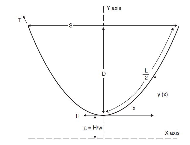
In these equations, $H$ is the cable traction at its center and $S$ is the total horizontal span. The relation $a = H/W$ is usually called the catenary constant. The mean traction can be approximated by $\bar{T} = (T+H)/2$, although the values $T$ and $H$ are usually quite close.
Now we define problem quantities, specifying the tension and calculating the sag such that it can be easily measured in the model.
g   =  9.81                         # local gravity (m/s^2)
S   =  100.                         # total spam (m)
H   =  5000.                        # cable tension at center (N)
phi =  0.0254                       # cable diameter (mm)
A   =  np.pi*((phi/2)**2)           # cross section nominal area (m^2)
Es  =  2.05e11                      # Young's modulus for steel (Pa)
ρs  =  7850.                        # density for steel (kg/m^3)

μL  =  ρs*A                         # mass per unit length (kg/m)
EA  =  Es*A                         # axial stiffness
D   =  μL*g*(S**2)/(8*H)            # cable sag (m)

print('Mass per unit length: {0:7.2f}kg/m.'.format(μL))
print('Axial stiffness:      {0:7.0f}kN.'.format(EA/1000))
print('Sag at center:        {0:7.2f}m.'.format(D))
Mass per unit length:    3.98kg/m.
Axial stiffness:       103875kN.
Sag at center:           9.76m.
The new base will be length, acceleration and density. This is an convenient approach for keeping the same gravity and designing the model to be tested in a wind tunnel.
ABC    = ['L', 'a', 'ρ']         # selected quantities for the new base
LMT    = ['L', 'M', 'T' ]        # dimensions are the last 3 columns of DimData
base   =  DimData.loc[ABC, LMT]  # the dimensional matrix
i_base =  np.linalg.inv(base)    # base inversion

λ_L    =  1/100                  # length scale for the reduced model
λ_a    =  1/1                    # acceleration remains unchanged (same gravity)
λ_ρ    =  1/1                    # imposed density (same fluid... air!)

base
| L | M | T | |
|---|---|---|---|
| L | 1 | 0 | 0 |
| a | 1 | 0 | -2 |
| ρ | -3 | 1 | 0 |
Let us calculate the scales for force, mass per unit length and time. Recall that he axial stiffness, $EA$, has the same scale as force.
par    = ['F', 'μL', 't']                    # selected scales to be calculated
npar   =  len(par)                           # number of quantities
DimMat =  DimData.loc[par, LMT]              # the dimensional matrix
scales =  np.tile([λ_L, λ_a, λ_ρ],(npar,1))  # prepare for calculations

DimMat
| L | M | T | |
|---|---|---|---|
| F | 1 | 1 | -2 |
| μL | -1 | 1 | 0 |
| t | 0 | 0 | 1 |
And finally the required scales are calculated.
NewMat = pd.DataFrame(data    = np.matmul(DimMat.values, i_base),
                      index   = DimMat.index,
                      columns = ABC)

[λ_F, λ_μL, λ_t]  = np.prod(scales**NewMat, axis=1);

print('Force (and axial stiffnees): λ_F  = 1:{0:7.0f}'.format(1/λ_F))
print('Mass per unit length:        λ_μL = 1:{0:7.0f}'.format(1/λ_μL))
print('Time:                        λ_t  = 1:{0:7.0f}'.format(1/λ_t))
Force (and axial stiffnees): λ_F  = 1:1000000
Mass per unit length:        λ_μL = 1:  10000
Time:                        λ_t  = 1:     10
The model mass per unit length must be:
μLM = λ_μL*μL

print('Model mass per unit length: {0:6.3f}g/m.'.format(1000*μLM))
Model mass per unit length: 0.398g/m.
If we take a nylon line, with Young's modulus $E = 3{\rm GPa}$ and density $\rho = 1150{\rm kg/m^3}$, the required diameter will be:
Eny = 3.00e9                    # nylon Young's modulus
ρny = 1150.0                    # nylon density

EAM = λ_F*EA
dM  = 2*np.sqrt((EAM/Eny)/np.pi)
AM  = np.pi*(dM/2)**2
μLM = ρny*AM

print('Nylon line diameter must be: {0:5.3f}mm.'.format(1000*dM))
print('Nylon line self weight is:   {0:5.3f}g/m.'.format(1000*μLM))
Nylon line diameter must be: 0.210mm.
Nylon line self weight is:   0.040g/m.
The nylon line self weight is not enough and the model mass per unit length may be completed with lead fishing beads. On the other hand, the cable axial deformation may be neglected and $EA$ regarded as infinity. In this case, any thin line with very small bending stiffness could be used, as long as the model mass is respected.
Finally, if the cable tension is to be measured, any load cell must be able to measure a force as small as:
HM = λ_F*H

print('Force balance in the range of... {0:6.4f}N.'.format(HM))
Force balance in the range of... 0.0050N.
However, if the cable is to be tested in a wind tunnel, the force measurement system must account for the expected load increase due to the aerodynamic drag.
2.3. Assignment 
- Defina um sistema estrutural simples, cuja resposta a uma dada carga possa ser calculada por uma fórmula teórica.
- Imagine um modelo reduzido para este sistema estrutural, escolha as grandezas que formarão a base dimensional, projete o modelo e calcule a resposta esperada no experimento.