Abstract: We have introduced you to the sequential process by which we decide to evaluation points in a simulation through Bayesian optimization. In this lecture we introduce Emukit. Emukit is a software framework for decision programming via surrogate modelling and emulation. It formalizes the process of selecting a point via an acquisition function and provides a general framework for incorporating surrogate models and the acquisition function of your choice. We’ll then show how Emukit can be used for active experimental design.
::: {.cell .markdown}
import matplotlib.pyplot as plt
plt.rcParams.update({'font.size': 22})
%pip install notutils
from the command prompt where you can access your python installation.
The code is also available on GitHub: https://github.com/lawrennd/notutils
Once notutils is installed, it can be imported in the usual manner.
import notutils
pods
[edit]
In Sheffield we created a suite of software tools for ‘Open Data Science’. Open data science is an approach to sharing code, models and data that should make it easier for companies, health professionals and scientists to gain access to data science techniques.
You can also check this blog post on Open Data Science.
The software can be installed using
%pip install pods
from the command prompt where you can access your python installation.
The code is also available on GitHub: https://github.com/lawrennd/ods
Once pods is installed, it can be imported in the usual manner.
import pods
%pip install mlai
from the command prompt where you can access your python installation.
The code is also available on GitHub: https://github.com/lawrennd/mlai
Once mlai is installed, it can be imported in the usual manner.
import mlai
%pip install gpy
%pip install pyDOE
%pip install emukit
Uncertainty Quantification and Design of Experiments
[edit]
We’re introducing you to the optimization and analysis of real-world models through emulation, this domain is part of a broader field known as surrogate modelling.
Although we’re approaching this from the machine learning perspective, with a computer-scientist’s approach, you won’t be surprised to find out that this field is not new and there are a diverse range of research communities interested in this domain.
We’ve been focussing on active experimental design. In particular, the case where we are sequentially selecting points to run our simulation based on previous results.
Here, we pause for a moment and cover approaches to passive experimental design. Almost all the emulation examples we’ve looked at so far need some initial points to ‘seed’ the emulator. Selecting these is also a task of experimental design, but one we perform without running our simulator.
This type of challenge, of where to run the simulation to get the answer you require is an old challenge. One classic paper, McKay et al. (1979), reviews three different methods for designing these inputs. They are random sampling, stratified sampling, and Latin hypercube sampling.
{Random sampling is the default approach, this is where across the input domain of interest, we just choose to select samples randomly (perhaps uniformly, or if we believe there’s an underlying distribution
Let the input values $\mathbf{ x}_1, \dots, \mathbf{ x}_n$ be a random sample from $f(\mathbf{ x})$. This method of sampling is perhaps the most obvious, and an entire body of statistical literature may be used in making inferences regarding the distribution of $Y(t)$.
In statistical surveillance stratified sampling is an approach from statistics where a population is divided into sub-populations before sampling. For example, imagine that we are interested surveillance data for Covid-19 tracking. If we can only afford to track 100 people, we could sample them randomly from across the population. But we might worry that (by chance) we don’t get many people from a particular age group. So instead, we could divide the population into sub-groups and sample a fixed number from each group. This ensures we get coverage across all ages, although downstream we might have to do some weighting of the samples when considering the population effect.
The same ideas can be deployed in emulation, your input domain can be divided into domains of particular intererest. For example if testing the performance of a component from an F1 car, you might be interested in the performance on the straight, the performance in “fast corners” and the performance in “slow corners”. Because slow corners have a very large effect on the final performance, you might take more samples from slow corners relative to the frequency that such corners appear in the actual races.
Using stratified sampling, all areas of the sample space of $\mathbf{ x}$ are represented by input values. Let the sample space $S$ of $\mathbf{ x}$ be partitioned into $I$ disjoint strata $S_t$. Let $\pi = P(\mathbf{ x}\in S_i)$ represent the size of $S_i$. Obtain a random sample $\mathbf{ x}_{ij}$, $j = 1, \dots, n$ from $S_i$. Then of course the $n_i$ sum to $n$. If $I = 1$, we have random sampling over the entire sample space.
Latin hypercube sampling is a form of stratified sampling. For a Latin square if $M$ samples are requred, then the strata are determined by dividing the area of the inputs into discrete $M$ rows and $M$ columns. Then the samples are taken so that each row and column only contains one total sample. The Latin hypercube is the generalisation of this idea to more than two dimensions.
The same reasoning that led to stratified sampling, ensuring that all portions of $S$ were sampled, could lead further. If we wish to ensure also that each of the input variables $\mathbf{ x}_k$ has all portions of its distribution represented by input values, we can divide the range of each $\mathbf{ x}_k$ into $n$ strata of equal marginal probability $1/n$, and sample once from each stratum. Let this sample be $\mathbf{ x}_{kj}$, $j = 1, \dots, n$. These form the $\mathbf{ x}_k$ component, $k = 1, \dots , K$, in $\mathbf{ x}_i$, $i = 1, \dots, n$. The components of the various $\mathbf{ x}_k$’s are matched at random. This method of selecting input values is an extension of quota sampling (Steinberg 1963), and can be viewed as a $K$-dimensional extension of Latin square sampling (Raj 1968).
The paper’s rather dated reference to “Output from a Computer Code” does carry forward through this literature, which has continued to be a focus of interest for statisticians. Tony O’Hagan, who was a colleague in Sheffield but is also one of the pioneers of Gaussian process models was developing these methods when I first arrived there (Kennedy and O’Hagan, 2001), and continued with a large EPSRC funded project for managing uncertainty in computational models, http://www.mucm.ac.uk/. You can see a list of their technical reports here.
Another important group based in France is the “MASCOT-NUM Research Group”, https://www.gdr-mascotnum.fr/. These researchers bring together statisticians, applied mathematicians and engineers in solving these problems.
Emukit
[edit]
The Emukit software we will be using across the next part of this module
is a python software library that facilitates emulation of systems. The
software’s origins go back to work done by Javier
Gonzalez as part of his
post-doctoral project at the University of Sheffield. Javier led the
design and build of a Bayesian optimization software. The package
GPyOpt worked with the SheffieldML software GPy for performing
Bayesian optimization.
GPyOpt had a modular design that allows the user to provide their own
surrogate models, the package was built with GPy as a surrogate model
in mind, but other surrogate models could also be wrapped and
integrated.
However, GPyOpt didn’t allow the full flexibility of surrogate
modelling for domains like experimental design, sensitivity analysis
etc.
Emukit (Paleyes et al., 2019) is designed and built for a more general
approach. The software is MIT licensed and its design and implementation
was led by Javier Gonzalez and Andrei
Paleyes at Amazon. Building
on the experience of GPyOpt, the aim with Emukit was to use the
modularisation ideas embedded in GPyOpt, but to extend them beyond the
modularisation of the surrogate models to modularisation of the
acquisition function.
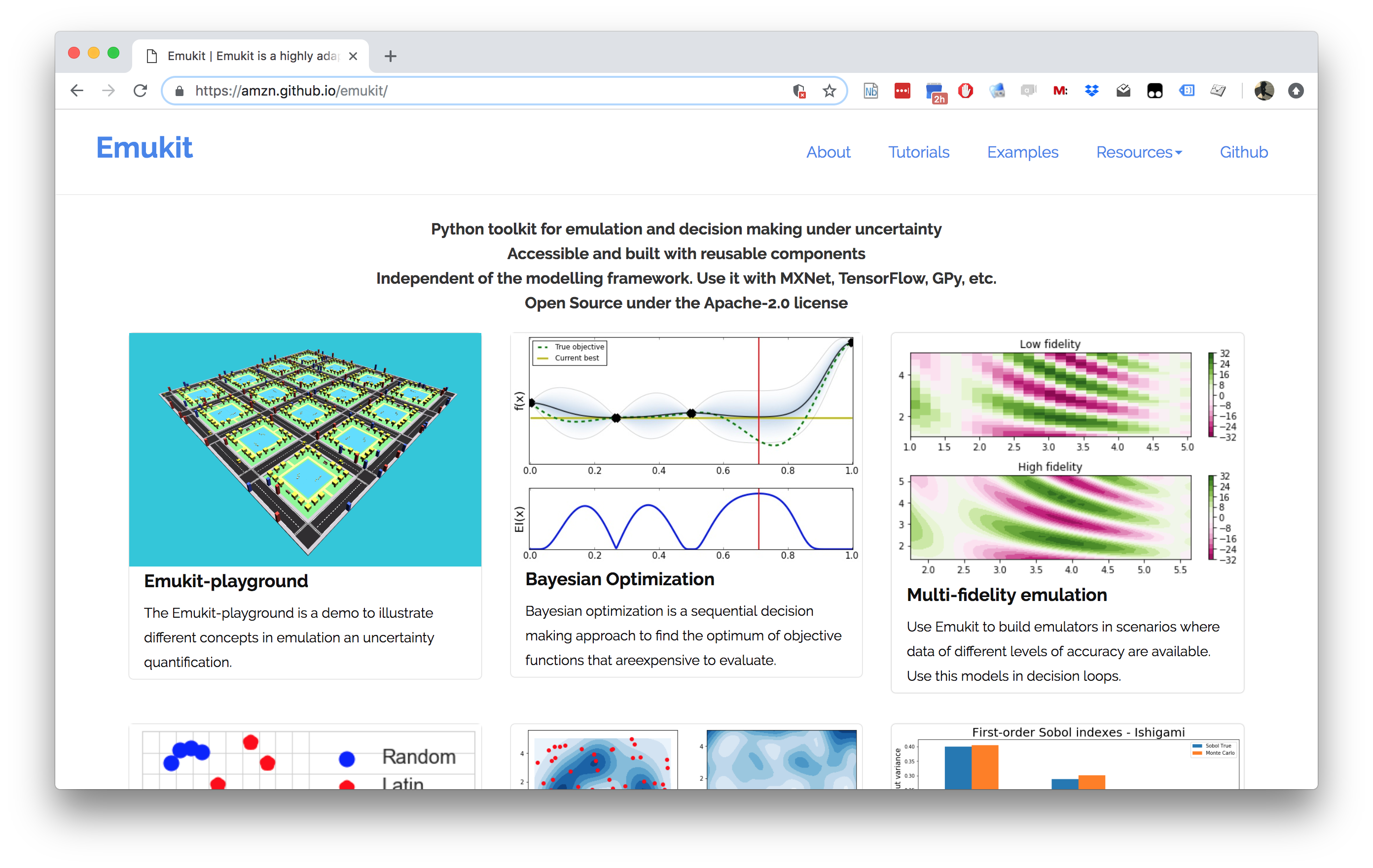
Figure: The Emukit software is a set of software tools for emulation and surrogate modeling. https://emukit.github.io/emukit/
To use Emukit you need a set of models to use as the surrogates, we’ll
use GPy.
Emukit does active experimental design, to access stratified sampling
and latin hypercube designs it makes use of the pyDOE package.
%pip install pyDOE
The software was initially built by the team in Amazon. As well as Javier Gonzalez (ML side) and Andrei Paleyes (Software Engineering) the team included Mark Pullin, Maren Mahsereci, Alex Gessner, Aaron Klein, Henry Moss, David-Elias Künstle as well as management input from Cliff McCollum and myself.
Emulation in Emukit
We see emulation comprising of three main parts:
Models. This is a probabilistic data-driven representation of the process/simulator that the user is working with. There is normally a modelling framework that is used to create a model. Examples: neural network, Gaussian process, random forest.
Methods. Relatively low-level techniques that are aimed that either understanding, quantifying or using uncertainty that the model provides. Examples: Bayesian optimization, experimental design.
Tasks. High level goals that owners of the process/simulator might be interested in. Examples: measure quality of a simulator, explain complex system behavior.
Typical workflow that we envision for a user interested in emulation is:
Figure out which questions/tasks are important for them in regard to their process/simulation.
Understand which emulation techniques are needed to accomplish the chosen task.
Build an emulator of the process. That can be a very involved step, that may include a lot of fine tuning and validation.
Feed the emulator to the chosen technique and use it to answer the question/complete the task.

Methods
This is the main focus of Emukit. Emukit defines a general structure of a decision-making method, called OuterLoop, and then offers implementations of few such methods: Bayesian optimization, experimental design. In addition to provide a framework for decision making Emukit provide other tools, like sensitivity analysis, that help to debug and interpret emulators. All methods in Emukit are model agnostic.
Models
Generally speaking, Emukit does not provide modelling capabilities, instead expecting users to bring their own models. Because of the variety of modelling frameworks out there, Emukit does not mandate or make any assumptions about a particular modelling technique or a library. Instead, it suggests to implement a subset of defined model interfaces required to use a particular method. Nevertheless, there are a few model-related functionalities in Emukit: - Example models, which give users something to play with to explore Emukit. - Model wrappers, which are designed to help adapting models in particular modelling frameworks to Emukit interfaces. - Multi-fidelity models, implemented based on GPy.
Tasks
Emukit does not contribute much to this part at the moment. However, the Emukit team are on lookout for typical use cases for Emukit, and if a reoccuring pattern emerges, it may become a part of the library.
while stopping condition is not met:
    optimize acquisition function
    evaluate user function
    update model with new observation
Emukit is built in a modular way so that each component in this loop can be swapped out. This means that scientists, applied mathematicians, machine learnings, statisticians can swap out the relevant part of their method and build on the underlying structure. You just need to pick out the part that requires implementation.
Loop
The emukit.core.loop.OuterLoop class is the abstract loop where the
different components come together. There are more specific loops for
Bayesian optimization and experimental design that construct some of the
component parts for you.
Model
All Emukit loops need a probabilistic model of the underlying system.
Emukit does not provide functionality to build models as there are
already many good modelling frameworks available in python. Instead, we
provide a way of interfacing third part modelling libraries with Emukit.
We already provide a wrapper for using a model created with GPy. For
instructions on how to include your own model please see this
notebook.
Different models and modelling frameworks will provide different
functionality. For instance, a Gaussian process will usually have
derivatives of the predictions available but random forests will not.
These different functionalities are represented by a set of interfaces
which a model implements. The basic interface that all models must
implement is IModel, which implements functionality to make
predictions and update the model but a model may implement any number of
other interfaces such as IDifferentiable which indicates a model has
prediction derivatives available.
Candidate Point Calculator
This class decides which point to evaluate next. The simplest
implementation, SequentialPointCalculator, collects one point at a
time by finding where the acquisition is a maximum by applying the
acquisition optimizer to the acquisition function. More complex
implementations will enable batches of points to be collected so that
the user function can be evaluated in parallel.
Acquisition
The acquisition is a heuristic quantification of how valuable collecting a future point might be. It is used by the candidate point calculator to decide which point(s) to collect next.
Acquisition Optimizer
The AcquisitionOptimizer optimizes the acquisition function to find
the point at which the acquisition is a maximum. This will use the
acquisition function gradients if they are available. If gradients of
the acquisition function are not available, it will either estimate them
numerically or use a gradient free optimizer.
User Function
This is the function that we are trying to reason about. It can be either evaluated by the user or it can be passed into the loop and evaluated by Emukit.
Model Updater
The ModelUpdater class updates the model with new training data after
a new point is observed and optimizes any hyper-parameters of the model.
It can decide whether hyper-parameters need updating based on some
internal logic.
Stopping Condition
The StoppingCondition class chooses when we should stop collecting
points. The most commonly used example is to stop when a set number of
iterations have been reached.
You can see more of Emukit being put into practice in this case study on Machine Learning in the Multiverse by Sam Bell.
import numpy as np
import GPy
Now set up Emukit to run.
from emukit.experimental_design.experimental_design_loop import ExperimentalDesignLoop
Let’s check the help function for the experimental design loop. This is the outer loop that provides all the decision making parts of Emukit.
ExperimentalDesignLoop?
Now let’s load in the model wrapper for our probabilistic model. In this case, instead of using GPy, we’ll make use of a simple model wrapper Emukit provides for a basic form of Gaussian process.
from emukit.model_wrappers import SimpleGaussianProcessModel
Let’s have a quick look at how the included GP model works.
SimpleGaussianProcessModel?
Now let’s create the data.
x_min = -30.0
x_max = 30.0

x = np.random.uniform(x_min, x_max, (10, 1))
y = np.sin(x) + np.random.randn(10, 1) * 0.05
To learn about how to include your own model in Emukit, check this
notebook
which shows how to include a sklearn GP model.
emukit_model = SimpleGaussianProcessModel(x, y)
from emukit.core import ParameterSpace, ContinuousParameter
from emukit.core.loop import UserFunctionWrapper
p = ContinuousParameter('c', x_min, x_max)
space = ParameterSpace([p])
loop = ExperimentalDesignLoop(space, emukit_model)
loop.run_loop(np.sin, 30)
plot_min = -40.0
plot_max = 40.0

real_x = np.arange(plot_min, plot_max, 0.2)
real_y = np.sin(real_x)
import matplotlib.pyplot as plt
import mlai.plot as plot
import mlai
fig, ax = plt.subplots(figsize=plot.big_wide_figsize)

ax.plot(real_x, real_y, c='r', linewidth=2)
ax.scatter(loop.loop_state.X[:, 0].tolist(),
           loop.loop_state.Y[:, 0].tolist(), s=50)

ax.set_xlabel('$x$')
ax.set_ylabel('$y$', rotation=None)
ax.set_ylim([-2.5, 2.5])

ax.legend(['true function', 'acquired data points'], loc='lower right')

mlai.write_figure('emukit-sine-function.svg', directory='./uq')

Figure: Experimental design in Emukit using the
ExperimentalDesignLoop: learning function $\sin(x)$ with Emukit.
Computer the predictions from the Emukit model.
predicted_y = []
predicted_std = []
for x in real_x:
    y, var = emukit_model.predict(np.array([[x]]))
    std = np.sqrt(var)
    predicted_y.append(y)
    predicted_std.append(std)

predicted_y = np.array(predicted_y).flatten()
predicted_std = np.array(predicted_std).flatten()
fig, ax = plt.subplots(figsize=plot.big_wide_figsize)

ax.plot(real_x, predicted_y, linewidth=3)
ax.plot(real_x, real_y, c='r', linewidth=2)

ax.set_ylim([-2.5, 2.5])

ax.fill_between(real_x, predicted_y - 2 * predicted_std,
                predicted_y + 2 * predicted_std, alpha=.5)

ax.set_xlabel('$x$')
ax.set_ylabel('$y$')
ax.legend(['true function', 'estimated function'], loc='lower right')

mlai.write_figure('emukit-sine-function-fit.svg', directory='./uq')

Figure: The fit to the sine function after runnning the Emukit
ExperimentalDesignLoop.
Exercise 1
Repeat the above experiment but using the Gaussian process model from
sklearn. You can see step by step instructions on how to do this in
this
notebook.
# Write your answer to Exercise 1 here
Emukit Overview Summary
The aim is to provide a suite where different approaches to emulation are assimilated under one roof. The current version of Emukit includes multi-fidelity emulation for build surrogate models when data is obtained from multiple information sources that have different fidelity and/or cost; Bayesian optimisation for optimising physical experiments and tune parameters of machine learning algorithms or other computational simulations; experimental design and active learning: design the most informative experiments and perform active learning with machine learning models; sensitivity analysis: analyse the influence of inputs on the outputs of a given system; and Bayesian quadrature: efficiently compute the integrals of functions that are expensive to evaluate. But it’s easy to extend.
This introduction is based on An Introduction to Experimental Design with Emukit written by Andrei Paleyes and Maren Mahsereci.
%pip install pyDOE
The pyDOE software is a python software package for design of experiments in python. It helps with model free experimental designs.
Approaches include Factorial Designs, Response Surface Designs and Randomized Designs. The software is hosted on Github https://github.com/tisimst/pyDOE/
https://pythonhosted.org/pyDOE/
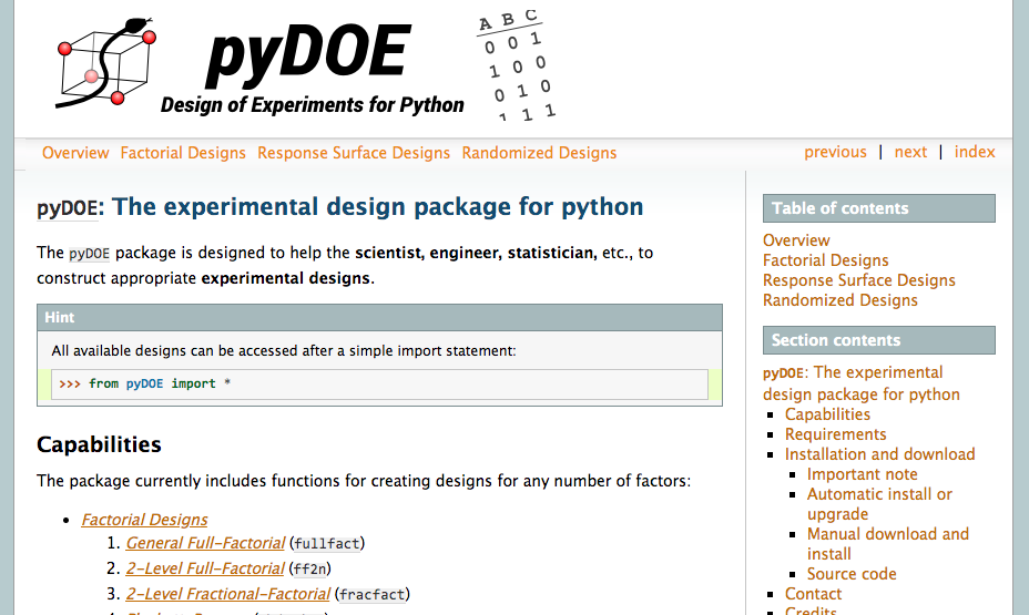
Figure: Design of Experiments for Python software. It provides various model free approaches to experimental design.
Alex Forrester
[edit]
We’re going to make use of the Forrester function in our example below, a function developed as a demonstrator by Alex Forrester. Alex is a design engineer who makes extensive use of surrogate modelling in Engineering design.
You can see Alex talking about the use of Gaussian process surrogates in this online video lecture.
from IPython.lib.display import YouTubeVideo
YouTubeVideo('2ngc2aw9xYs')
Figure: A kinematic simulation of the human body doing breaststroke that Alex uses as part of his work in optimization of human motion during sports.
The Forrester function (Forrester et al., 2008) is commonly used as a demonstrator function in surrogate modelling. It has the form $$ f(x) = (6x-2)^2\sin(12 x-4). $$
import numpy as np
x = np.linspace(0, 1, 100)
f = (6*x-2)**2 * np.sin(12*x-4)
import matplotlib.pyplot as plt
import mlai.plot as plot
import mlai
fig, ax = plt.subplots(figsize=plot.big_wide_figsize)
ax.plot(x, f, 'r-', linewidth=2)
ax.set_xlabel('$x$')
ax.set_ylabel('$f(x)$')
ax.set_xlim(-0.01, 1)
ax.set_ylim([-20, 20])

mlai.write_figure('forrester-function.svg', directory='./uq')

Figure: The Forrester function is commonly used as an exemplar function for surrogate modelling and emulation. It has the form $f(x) = (6x-2)^2\sin(12 x-4)$
We’re going to introduce the experimental design acquisition functions by looking at the Forrester function (Forrester et al., 2008)
import numpy as np

from emukit.test_functions import forrester_function
#from emukit.core.loop.user_function import UserFunctionWrapper
#from emukit.core import ContinuousParameter, ParameterSpace
target_function, space = forrester_function()
x_plot = np.linspace(space.parameters[0].min, space.parameters[0].max, 301)[:, None]
y_plot = target_function(x_plot)
fig, ax = plt.subplots(figsize=plot.big_wide_figsize)
ax.plot(x_plot, y_plot, 'k', label='target Function', linewidth=2)

ax.legend(loc=2)
ax.set_xlabel('$x$')
ax.set_ylabel('$f(x)$')
ax.grid(True)
ax.set_xlim(0, 1)

mlai.write_figure(filename='forrester-function.svg', directory='./uq')
Figure: The Forrester function (Forrester et al., 2008).
Initial Design
Usually, before we start the actual ExpDesign loop we need to gather a
few observations such that we can fit the model. This is called the
initial design and common strategies are either a predefined grid or
sampling points uniformly at random. These strategies are known as
model-free experimental design.
X_init = np.array([[0.2],[0.6], [0.9]])
Y_init = target_function(X_init)
fig, ax = plt.subplots(figsize=plot.big_wide_figsize)
ax.plot(X_init, Y_init, 'ro', markersize=10, label='observations')
ax.plot(x_plot, y_plot, 'k', label='target Function', linewidth=2)

ax.legend(loc=2)
ax.set_xlabel('$x$')
ax.set_ylabel('$f(x)$')
ax.grid(True)
ax.set_xlim(-0.01, 1)
ax.set_ylim([-20, 20])

mlai.write_figure(filename='forrester-function-initial-design.svg', directory='./uq')

Figure: The initial design for the Forrester function example.
The Model
Now we can start with the ExpDesign loop by first fitting a model on
the collected data. A popular model for ExpDesign is a Gaussian
process (GP) which defines a probability distribution across classes of
functions, typically smooth, such that each linear finite-dimensional
restriction is multivariate Gaussian (Rasmussen and Williams, 2006).
Gaussian processes are fully parametrized by a mean $\mu(\mathbf{ x})$
and a covariance function $k(\mathbf{ x},\mathbf{ x}^\prime)$. Without
loss of generality $\mu(\mathbf{ x})$ is assumed to be zero. The
covariance function $k(\mathbf{ x},\mathbf{ x}^\prime)$ characterizes
the smoothness and other properties of $f$. It is known that the kernel
of the process has to be continuous, symmetric and positive definite. A
widely used kernel is the exponentiated quadratic or RBF kernel: $$
k(\mathbf{ x},\mathbf{ x}^\prime) = \alpha \exp{ \left(-\frac{\|\mathbf{ x}-\mathbf{ x}^\prime\|^2}{2 \ell}\right)}
$$ where $\alpha$ and $\ell$ are hyperparameters.
To denote that $f$ is a sample from a GP with mean $\mu$ and covariance $k$ we write $$ f\sim \mathcal{GP}(\mu,k). $$
For regression tasks, the most important feature of GPs is that process priors are conjugate to the likelihood from finitely many observations $\mathbf{Y}= (y_1,\dots,y_n)^\top$ and $\mathbf{X}=\{\mathbf{ x}_1,\dots,\mathbf{ x}_n\}$, $\mathbf{ x}_i\in \mathcal{X}$ of the form $y_i = f(\mathbf{ x}_i) + \epsilon_i$ where $\epsilon_i \sim \mathcal{N}\left(0,\sigma^2\right)$ and we typically estimate $\sigma^2$ by maximum likelihood alongside $\alpha$ and $\ell$.
We obtain the Gaussian posterior $$ f(\mathbf{ x}^*)|\mathbf{X}, \mathbf{Y}, \theta \sim \mathcal{N}\left(\mu(\mathbf{ x}^*),\sigma^2(\mathbf{ x}^*)\right), $$ where $\mu(\mathbf{ x}^*)$ and $\sigma^2(\mathbf{ x}^*)$ have a closed form solution as we’ve seen in the earlier lectures (see also Rasmussen and Williams (2006)).
Note that Gaussian processes are also characterized by hyperparameters, for example in the exponentiated quadratic case we have $\boldsymbol{ \theta}= \left\{ \alpha, \ell, \sigma^2 \right\}$ for the scale of the covariance, the lengthscale and the noise variance. Here, for simplicity we will keep these hyperparameters fixed. However, we will usually either optimize or sample these hyperparameters using the marginal loglikelihood of the GP.
In this module we’ve focussed on Gaussian processes, but we could also
use any other model that returns a mean $\mu(\mathbf{ x})$ and variance
$\sigma^2(\mathbf{ x})$ on arbitrary input points $\mathbf{ x}$ such as
Bayesian neural networks or random forests. In Emukit these different
models can also be used by defining a new ModelWrapper.
Here we’re going to wrap a GPy model.
import GPy
from emukit.model_wrappers.gpy_model_wrappers import GPyModelWrapper
Now we set up the covariance function for the GPy model, initialising it with a lengthscale, $\ell=0.08$, and a variance, $\alpha=20$.
kern = GPy.kern.RBF(1, lengthscale=0.08, variance=20)
gpy_model = GPy.models.GPRegression(X_init, Y_init, kern, noise_var=1e-10)
emukit_model = GPyModelWrapper(gpy_model)

mu_plot, var_plot = emukit_model.predict(x_plot)
import matplotlib.pyplot as plt

from matplotlib import colors as mcolors
from matplotlib import cm

colors = dict(mcolors.BASE_COLORS, **mcolors.CSS4_COLORS)
def helper_plot_emulator_errorbars():
    """Helper function for plotting the emulator fit."""
    ax.plot(emukit_model.X, emukit_model.Y, 'ro', markersize=10, label='observations')
    ax.plot(x_plot, mu_plot, 'C0', label='model', linewidth=3)
    ax.plot(x_plot, y_plot, 'k', label='target function', linewidth=2)
    ax.fill_between(x_plot[:, 0],
                 mu_plot[:, 0] + np.sqrt(var_plot)[:, 0],
                 mu_plot[:, 0] - np.sqrt(var_plot)[:, 0], color='C0', alpha=0.6)
    ax.fill_between(x_plot[:, 0],
                 mu_plot[:, 0] + 2 * np.sqrt(var_plot)[:, 0],
                 mu_plot[:, 0] - 2 * np.sqrt(var_plot)[:, 0], color='C0', alpha=0.4)
    ax.fill_between(x_plot[:, 0],
                 mu_plot[:, 0] + 3 * np.sqrt(var_plot)[:, 0],
                 mu_plot[:, 0] - 3 * np.sqrt(var_plot)[:, 0], color='C0', alpha=0.2)
    ax.legend(loc=2)
    ax.set_xlabel('$x$')
    ax.set_ylabel('$f(x)$')
    ax.grid(True)
    ax.set_xlim(-0.01, 1)
    ax.set_ylim([-20, 20])
fig, ax = plt.subplots(figsize=plot.big_wide_figsize)
helper_plot_emulator_errorbars()
mlai.write_figure(filename='forrester-function-multi-errorbars-00.svg', directory='./uq')

Figure: The emulator fitted to the Forrester function with only three observations from the inital design. The error bars show 1, 2 and 3 standard deviations.
The Acquisition Function
In the second step of our ExpDesign loop we use our model to compute the acquisition function. We’ll review two different forms of acquisition funciton for doing this.
Uncertainty Sampling
In uncertainty sampling (US) we hoose the next value $\mathbf{ x}_{n+1}$ at the location where the model on $f(\mathbf{ x})$ has the highest marginal predictive variance $$ a_{US}(\mathbf{ x}) = \sigma^2(\mathbf{ x}). $$ This makes sure, that we learn the function $f(\cdot)$ everywhere on $\mathbb{X}$ to a similar level of absolute error.
Integrated Variance Reduction
In the integrated variance reduction (IVR) you choose the next value $\mathbf{ x}_{n+1}$ such that the total variance of the model is reduced maximally (Sacks et al., 1989), $$ \begin{align*} a_{\text{IVR}} & = \int_{\mathbb{X}}[\sigma^2(\mathbf{ x}') - \sigma^2(\mathbf{ x}'; \mathbf{ x})]\text{d}\mathbf{ x}' \\ & \approx \frac{1}{\# \text{samples}}\sum_i^{\# \text{samples}}[\sigma^2(\mathbf{ x}_i) - \sigma^2(\mathbf{ x}_i; \mathbf{ x})]. \end{align*} $$ Here $\sigma^2(\mathbf{ x}'; \mathbf{ x})$ is the predictive variance at $\mathbf{ x}'$ had $\mathbf{ x}$ been observed. Thus IVR computes the overall reduction in variance (for all points in $\mathbb{X}$) had $f$ been observed at $\mathbf{ x}$.
The finite sum approximation on the right-hand side of the equation is usually used because the integral over $\mathbf{ x}'$ is not analytic. In that case $\mathbf{ x}_i$ are sampled randomly. For a GP model the right-hand side simplifies to
$$ a_{LCB} \approx \frac{1}{\# \text{samples}}\sum_i^{\# \text{samples}}\frac{k^2(\mathbf{ x}_i, \mathbf{ x})}{\sigma^2(\mathbf{ x})}. $$IVR is arguably the more principled approach, but often US is preferred over IVR simply because it lends itself to gradient based optimization more easily, is cheaper to compute, and is exact.
For both of them (stochastic) gradient base optimizers are used to retrieve $\mathbf{ x}_{n+1} \in \operatorname*{arg\:max}_{\mathbf{ x}\in \mathbb{X}} a(\mathbf{ x})$.
from emukit.experimental_design.acquisitions import IntegratedVarianceReduction, ModelVariance
us_acquisition = ModelVariance(emukit_model)
ivr_acquisition = IntegratedVarianceReduction(emukit_model, space)

us_plot = us_acquisition.evaluate(x_plot)
ivr_plot = ivr_acquisition.evaluate(x_plot)
fig, ax = plt.subplots(figsize=plot.big_wide_figsize)
ax.plot(x_plot, us_plot / np.max(us_plot), 'green', label='US', linewidth=3)
ax.plot(x_plot, ivr_plot / np.max(ivr_plot) , 'purple', label='IVR', linewidth=3)

ax.legend(loc=1)
ax.set_xlabel('$x$')
ax.set_ylabel('$f(x)$')
ax.grid(True)
ax.set_xlim(-0.01, 1)

mlai.write_figure('experimental-design-acquisition-forrester-00.svg', directory='./uq')

Figure: The uncertainty sampling and integrated variance reduction acquisition functions for the Forrester example.
Evaluating the objective function
To find the next point to evaluate we optimize the acquisition function using a standard gradient descent optimizer.
def helper_plot_next_point_acquisition():
    """Helper code for plot the location of the next point acquisition."""
    ax.plot(x_plot, us_plot / np.max(us_plot), 'green', label='US', linewidth=3)
    ax.axvline(x_new, color='red', label='x_next', linestyle='--', linewidth=3)
    ax.legend(loc=1)
    ax.set_xlabel('$x$')
    ax.set_ylabel('$f(x)$')
    ax.grid(True)
    ax.set_xlim(-0.01, 1)
from emukit.core.optimization import GradientAcquisitionOptimizer
optimizer = GradientAcquisitionOptimizer(space)
x_new, _ = optimizer.optimize(us_acquisition)
fig, ax = plt.subplots(figsize=plot.big_wide_figsize)
helper_plot_next_point_acquisition()
mlai.write_figure('experimental-design-acquisition-forrester-01.svg', directory='./uq')

Figure: The maxima of the acquisition function is found and this point is selected for inclusion.
Afterwards we evaluate the true objective function and append it to our initial observations.
y_new = target_function(x_new)
X = np.append(X_init, x_new, axis=0)
Y = np.append(Y_init, y_new, axis=0)
After updating the model, you can see that the uncertainty about the true objective function in this region decreases and our model becomes more certain.
emukit_model.set_data(X, Y)
mu_plot, var_plot = emukit_model.predict(x_plot)
fig, ax = plt.subplots(figsize=plot.big_wide_figsize)
helper_plot_emulator_errorbars()

mlai.write_figure(filename='forrester-function-multi-errorbars-01.svg', directory='./uq')

Figure: The target Forrester function plotted alongside the emulation model and error bars from the emulation at 1, 2 and 3 standard deviations.
We can repeat this process to obtain more points.
us_acquisition = ModelVariance(emukit_model)
us_plot = us_acquisition.evaluate(x_plot)
x_new, _ = optimizer.optimize(us_acquisition)
fig, ax = plt.subplots(figsize=plot.big_wide_figsize)
helper_plot_next_point_acquisition()

mlai.write_figure('experimental-design-acquisition-forrester-02.svg', directory='./uq')

Figure: The maxima of the acquisition function is found and this point is selected for inclusion.
Once again we can asimmilate the new target function observation into the model and re-evaluate our emulation.
y_new = target_function(x_new)
X = np.append(X, x_new, axis=0)
Y = np.append(Y, y_new, axis=0)
emukit_model.set_data(X, Y)
mu_plot, var_plot = emukit_model.predict(x_plot)
Resulting in an updated estimate of the function.
fig, ax = plt.subplots(figsize=plot.big_wide_figsize)
helper_plot_emulator_errorbars()

mlai.write_figure(filename='forrester-function-multi-errorbars-02.svg', directory='./uq')

Figure: The target Forrester function plotted alongside the emulation model and error bars from the emulation at 1, 2 and 3 standard deviations.
Emukit’s Experimental Design Interface
Of course in practice we don’t want to implement all of these steps our self. Emukit provides a convenient and flexible interface to apply experimental design. Below we can see how to run experimental design on the exact same function for 10 iterations.
from emukit.experimental_design.experimental_design_loop import ExperimentalDesignLoop
ed = ExperimentalDesignLoop(space=space, model=emukit_model)

ed.run_loop(target_function, 10)
mu_plot, var_plot = ed.model.predict(x_plot)
fig, ax = plt.subplots(figsize=plot.big_wide_figsize)
helper_plot_emulator_errorbars()

mlai.write_figure(filename='forrester-function-full-fit.svg', directory='./uq')

Figure: The fit of the model to the Forrester function.
Conclusions
We’ve introduced the Emukit software and outlined its design philosophy. We’ve then performed some simple examples using Emukit to perform experimental design as a task. In particular we saw how we could define the task as an acquisition funciton, a loop, an emulator model and a target function.
You can compare the design of this software with its predecessor,
GPyOpt, which is less modular in its design, and more focussed on
Bayesian optimization.
Thanks!
For more information on these subjects and more you might want to check the following resources.
- twitter: @lawrennd
- podcast: The Talking Machines
- newspaper: Guardian Profile Page
- blog: http://inverseprobability.com
References
Forrester, A.I.J., Sóbester, A., Keane, A.J., 2008. Engineering design via surrogate modelling: A practical guide. wiley. https://doi.org/10.1002/9780470770801
Kennedy, M.C., O’Hagan, A., 2001. Bayesian calibration of computer models. Journal of the Royal Statistical Society: Series B (Statistical Methodology) 63, 425–464. https://doi.org/10.1111/1467-9868.00294
McKay, M.D., Beckman, R.J., Conover, W.J., 1979. A comparison of three methods for selecting values of input variables in the analysis of output from a computer code. Technometrics 21, 239–245.
Paleyes, A., Pullin, M., Mahsereci, M., McCollum, C., Lawrence, N.D., Gonzalez, J., 2019. Emulation of physical processes with emukit, in: Second Workshop on Machine Learning and the Physical Sciences, NeuRIPS 2019.
Rasmussen, C.E., Williams, C.K.I., 2006. Gaussian processes for machine learning. mit, Cambridge, MA.
Sacks, J., Welch, W.J., Mitchell, T.J., Wynn, H.P., 1989. Design and analysis of computer experiments. Statistical Science 4, 409–423. https://doi.org/10.1214/ss/1177012413