Introducción a Python para ciencias e ingenierías (notebook 4)
Ing. Martín Gaitán
Twitter: @tin_nqn_
** Registrá tu asistencia a esta clase **
http://goo.gl/forms/olbkNwX700
Links útiles
Repositorio del curso:
http://bit.ly/cursopy
Python "temporal" online:
http://try.jupyter.org
- Descarga de Python "Anaconda"
- Resumen de sintaxis markdown
Matplotlib, un gráfico vale más que mil palabras
Python es un lenguaje muy completo pero, aunque es muy grande, su librería estándar no es infinita. Por suerte hay miles y miles de bibliotecas extras para complementar casi cualquier aspecto en el que queramos aplicar Python. En algunos ámbitos, con soluciones muy destacadas.
Para hacer gráficos la opción canónica es Matplotlib http://matplotlib.org/ . Ya viene instalado con la versión completa de Anaconda.
%matplotlib inline
from matplotlib import pyplot # generalmente importado "as plt"
x = [0.1*i for i in range(-50, 51)]
x
[-5.0,
 -4.9,
 -4.800000000000001,
 -4.7,
 -4.6000000000000005,
 -4.5,
 -4.4,
 -4.3,
 -4.2,
 -4.1000000000000005,
 -4.0,
 -3.9000000000000004,
 -3.8000000000000003,
 -3.7,
 -3.6,
 -3.5,
 -3.4000000000000004,
 -3.3000000000000003,
 -3.2,
 -3.1,
 -3.0,
 -2.9000000000000004,
 -2.8000000000000003,
 -2.7,
 -2.6,
 -2.5,
 -2.4000000000000004,
 -2.3000000000000003,
 -2.2,
 -2.1,
 -2.0,
 -1.9000000000000001,
 -1.8,
 -1.7000000000000002,
 -1.6,
 -1.5,
 -1.4000000000000001,
 -1.3,
 -1.2000000000000002,
 -1.1,
 -1.0,
 -0.9,
 -0.8,
 -0.7000000000000001,
 -0.6000000000000001,
 -0.5,
 -0.4,
 -0.30000000000000004,
 -0.2,
 -0.1,
 0.0,
 0.1,
 0.2,
 0.30000000000000004,
 0.4,
 0.5,
 0.6000000000000001,
 0.7000000000000001,
 0.8,
 0.9,
 1.0,
 1.1,
 1.2000000000000002,
 1.3,
 1.4000000000000001,
 1.5,
 1.6,
 1.7000000000000002,
 1.8,
 1.9000000000000001,
 2.0,
 2.1,
 2.2,
 2.3000000000000003,
 2.4000000000000004,
 2.5,
 2.6,
 2.7,
 2.8000000000000003,
 2.9000000000000004,
 3.0,
 3.1,
 3.2,
 3.3000000000000003,
 3.4000000000000004,
 3.5,
 3.6,
 3.7,
 3.8000000000000003,
 3.9000000000000004,
 4.0,
 4.1000000000000005,
 4.2,
 4.3,
 4.4,
 4.5,
 4.6000000000000005,
 4.7,
 4.800000000000001,
 4.9,
 5.0]
y = [x_i**2 for x_i in x]
y
[25.0,
 24.010000000000005,
 23.040000000000006,
 22.090000000000003,
 21.160000000000004,
 20.25,
 19.360000000000003,
 18.49,
 17.64,
 16.810000000000006,
 16.0,
 15.210000000000003,
 14.440000000000001,
 13.690000000000001,
 12.96,
 12.25,
 11.560000000000002,
 10.890000000000002,
 10.240000000000002,
 9.610000000000001,
 9.0,
 8.410000000000002,
 7.840000000000002,
 7.290000000000001,
 6.760000000000001,
 6.25,
 5.760000000000002,
 5.290000000000001,
 4.840000000000001,
 4.41,
 4.0,
 3.6100000000000003,
 3.24,
 2.8900000000000006,
 2.5600000000000005,
 2.25,
 1.9600000000000004,
 1.6900000000000002,
 1.4400000000000004,
 1.2100000000000002,
 1.0,
 0.81,
 0.6400000000000001,
 0.4900000000000001,
 0.3600000000000001,
 0.25,
 0.16000000000000003,
 0.09000000000000002,
 0.04000000000000001,
 0.010000000000000002,
 0.0,
 0.010000000000000002,
 0.04000000000000001,
 0.09000000000000002,
 0.16000000000000003,
 0.25,
 0.3600000000000001,
 0.4900000000000001,
 0.6400000000000001,
 0.81,
 1.0,
 1.2100000000000002,
 1.4400000000000004,
 1.6900000000000002,
 1.9600000000000004,
 2.25,
 2.5600000000000005,
 2.8900000000000006,
 3.24,
 3.6100000000000003,
 4.0,
 4.41,
 4.840000000000001,
 5.290000000000001,
 5.760000000000002,
 6.25,
 6.760000000000001,
 7.290000000000001,
 7.840000000000002,
 8.410000000000002,
 9.0,
 9.610000000000001,
 10.240000000000002,
 10.890000000000002,
 11.560000000000002,
 12.25,
 12.96,
 13.690000000000001,
 14.440000000000001,
 15.210000000000003,
 16.0,
 16.810000000000006,
 17.64,
 18.49,
 19.360000000000003,
 20.25,
 21.160000000000004,
 22.090000000000003,
 23.040000000000006,
 24.010000000000005,
 25.0]
pyplot.plot(x,y)
[<matplotlib.lines.Line2D at 0x7fa2d5b495f8>]

Los gráficos emergentes son buenos porque tiene la barra de herramientas (interactividad) y podemos guardarlos en excelente calidad a golpe de mouse. Pero en los notebooks podemos poner los gráficos directamente incrustados
%matplotlib inline
pyplot.plot(x,y)
pyplot.title('Pará bola!')
pyplot.scatter([0, 2], [15, 25])
pyplot.annotate(s='un punto', xy=(0, 15), xytext=(0.3, 15.2))
pyplot.annotate(s='otro un punto', xy=(2, 25), xytext=(2.3, 25.2))
pyplot.grid()

Matplotlib sabe hacer muchísimos tipos de gráficos!
!cat data/near_critical_oil.csv
Component,Mol fraction
n2,0.46
co2,3.36
c1,62.36
c2,8.9
c3,5.31
c4,3.01
c5,1.5
c6,1.05
c7,2.0
c7+,12.049
import csv

with open('data/near_critical_oil.csv') as csv_file:
    reader = csv.reader(csv_file)
    critical_oil = [line for line in reader]   #o list(reader)

components = [c for (c, f) in critical_oil[1:]]
fraction = [float(f) for (c, f) in critical_oil[1:]]
# el ; evita el output de la celda
pyplot.pie(fraction, labels=components, shadow=True);

import random
campana = [random.gauss(0, 0.5) for i in range(1000)]
pyplot.hist(campana, bins=15);

La "papa" de matplotlib
Este es el algoritmo más importante para graficar con matplotlib
- Ir a http://matplotlib.org/gallery
- Elegir el gráfico de ejemplo que más se parezca a lo que queremos lograr
- Copiar el código del ejemplo y adaptarlo a nuestros datos y gustos

import numpy as np
import matplotlib.pyplot as plt


N = 20
theta = np.linspace(0.0, 2 * np.pi, N, endpoint=False)
radii = 10 * np.random.rand(N)
width = np.pi / 4 * np.random.rand(N)

ax = plt.subplot(111, projection='polar')
bars = ax.bar(theta, radii, width=width, bottom=0.0)

# Use custom colors and opacity
for r, bar in zip(radii, bars):
    bar.set_facecolor(plt.cm.jet(r / 10.))
    bar.set_alpha(0.5)

plt.show()

Ejercicios
- Dada la función para el cálculo de raices de una ecuación de segundo grado implementada en clases anteriores, crear una función que dados los coeficientes grafique la parábola y denote las raices con puntos rojos y el valor de X en cada una.
- Basado en el ejemplo de grafico de torta de la galería, adaptar el ejemplo que grafica "near_critical_oil.csv" para que no se vea "ovoide" y la porción correspondiente a "C2" quede separada. Agregar un título al gráfico
# %load https://gist.githubusercontent.com/mgaitan/f0ceedbc1890038cf27f/raw/48fe60095644647d8b5b084b60547b4da0751201/plot_parabola.py
def baskara(a, b=0, c=0):
    """dados los coeficientes, encuentra los valores de x tal que ax^2 + bx + c = 0"""

    discriminante = (b**2 - 4*a*c)**0.5
    x1 = (-b + discriminante)/(2*a)
    x2 = (-b - discriminante)/(2*a)
    return (x1, x2)


def plot_parabola(a, b=0, c=0):
    X = [.1 * i for i in range(-50, 51)]
    Y = [(a*x**2 + b*x + c)  for x in X]
    pyplot.plot(X,Y)
    pyplot.plot(x, [0 for x in X], linestyle='dashed')
    pyplot.title('un titulo')
    x1, x2 = baskara(a, b, c)
    if not isinstance(x1, complex):
        pyplot.scatter([x1, x2], [0, 0], color='red')
        pyplot.annotate(s=round(x1, 2), xy=(x1, 0), xytext=(x1+0.3, .2))
        pyplot.annotate(s=round(x2, 2), xy=(x2, 0), xytext=(x2 + .3, .2))


plot_parabola(1.2, b=0.4, c=-1.4)

import csv

with open('data/near_critical_oil.csv') as csv_file:
    reader = csv.reader(csv_file)
    critical_oil = [line for line in reader]   #o list(reader)

components = [c for (c, f) in critical_oil[1:]]
fraction = [float(f) for (c, f) in critical_oil[1:]]
explode = [0.2 if c == 'c2' else 0 for c in components]
# el ; evita el output de la celda

pyplot.pie(fraction, explode=explode, labels=components, shadow=True)
pyplot.axis('equal');

Antes de seguir con Matplotlib debemos aprender el corazón del Python Cientifico: Numpy
Numpy, todo es un array
El paquete numpy es usado en casi todos los cálculos numéricos usando Python. Es un paquete que provee a Python de estructuras de datos vectoriales, matriciales y de rango mayor, de alto rendimiento. Está implementado en C y Fortran, de modo que cuando los cálculos son vectorizados (formulados con vectores y matrices), el rendimiento es muy bueno.
import numpy as np
El pilar de numpy (y toda la computación científica basada en Python) es el tipo de datos ndarray, o sea arreglos de datos multidimensionales.
¿Otra secuencia más? ¿pero que tenían de malo las listas?
Las listas son geniales paro guardar cualquier tipo de objeto, pero esa flexibilidad las vuelve ineficientes cuando lo que queremos es almacenar datos homogéneos
%timeit [0.1*i for i in range(10000)] # %timeit es otra magia de ipython
1000 loops, best of 3: 1.08 ms per loop
%timeit np.arange(0, 1000, .1) # arange es igual a range, pero soporta paso de tipo flotante y devuelve un array
The slowest run took 13.32 times longer than the fastest. This could mean that an intermediate result is being cached
10000 loops, best of 3: 38.2 µs per loop
%%timeit -o
X = range(10000000)
Y = range(10000000)
Z = [(x + y) for x,y in zip(X,Y)]
1 loops, best of 3: 991 ms per loop
<TimeitResult : 1 loops, best of 3: 991 ms per loop>
%%timeit -o
X = np.arange(10000000)
Y = np.arange(10000000)
Z = X + Y
10 loops, best of 3: 156 ms per loop
<TimeitResult : 10 loops, best of 3: 156 ms per loop>
__.best / _.best
6.370105952818687
Existen varias formas para inicializar nuevos arrays de numpy, por ejemplo desde
- Listas o tuplas
- Usando funciones dedicadas a generar arreglos numpy, como
arange,linspace,ones,zerosetc. - Leyendo datos desde archivos
v = np.array([1,2,3,4])
v
array([1, 2, 3, 4])
# una matriz: el argumento de la función array function es una lista anidada de Python
M = np.array([[1, 2],
              [3, 4.0]])
M
array([[ 1.,  2.],
       [ 3.,  4.]])
type(v), type(M)
(numpy.ndarray, numpy.ndarray)
Dimensiones, tamaño, tipo, forma
Los ndarrays tienen distintos atributos. Por ejemplo
v.ndim, M.ndim # cantidad de dimensiones
(1, 2)
v.shape, M.shape # tupla de "forma". len(v.shape) == v.ndim
((4,), (2, 2))
v.size, M.size # cantidad de elementos.
(4, 4)
M.T # transpuesta!
array([[1, 3],
       [2, 4]])
A diferencia de las listas, los arrays tambien tienen un tipo homogéneo
v.dtype, M.dtype #
(dtype('int64'), dtype('float64'))
Se puede definir explicitamente el tipo de datos del array
np.array([[1, 2], [3, 4]], dtype=complex)
---------------------------------------------------------------------------
TypeError                                 Traceback (most recent call last)
<ipython-input-36-737d9df13f43> in <module>()
----> 1 np.array([[1, 2], [3, 'f']], dtype=complex)

TypeError: a float is required
Una gran ventaja del atributo shape es que podemos cambiarlo. Es decir, reacomodar la distrución de los elementos (por supuesto, sin perderlos en el camino)
A = np.arange(0, 12)
A.shape
(12,)
A.shape = 3, 4
A
array([[ 0,  1,  2,  3],
       [ 4,  5,  6,  7],
       [ 8,  9, 10, 11]])
El método reshape es otra manera de definir la forma de un array, generando uno nuevo array (a diferencia de A.shape que simplemente es otra vista del mismo array)
A = np.arange(12).reshape((3,4))
A
array([[ 0,  1,  2,  3],
       [ 4,  5,  6,  7],
       [ 8,  9, 10, 11]])
Vistas
Esto es porque numpy en general no mueve los elementos de la memoria y en cambio usa vistas para mostrar los elementos de distinta forma. Es importante entender esto porque incluso los slicings son vistas.
a = np.arange(10)
a
array([0, 1, 2, 3, 4, 5, 6, 7, 8, 9])
a = np.arange(10)
b = a[::2]  # todo de 2 en 2
b
array([0, 2, 4, 6, 8])
b[0] = 12
a  # chan!!!
array([12, 1, 2, 3, 4, 5, 6, 7, 8, 9])
En cambio
c = np.arange(10)
d = c[::2].copy()
d[0] = 12
c
array([0, 1, 2, 3, 4, 5, 6, 7, 8, 9])
Una forma de saber si un array es "base" o hereda los datos de otro array (es una vista), es verificar el atributo base
b.base is a and a.base is None
True
Otras funciones constructuras de arrays
Además de arange hay otras funciones que devuelven arrays. Por ejemplo linspace, que a diferencia de arange no se da el tamaño del paso, sino la cantidad de puntos que queremos en el rango
np.linspace(0, 2 * np.pi, 100) # por defecto, incluye el limite.
array([ 0.        ,  0.06346652,  0.12693304,  0.19039955,  0.25386607,
        0.31733259,  0.38079911,  0.44426563,  0.50773215,  0.57119866,
        0.63466518,  0.6981317 ,  0.76159822,  0.82506474,  0.88853126,
        0.95199777,  1.01546429,  1.07893081,  1.14239733,  1.20586385,
        1.26933037,  1.33279688,  1.3962634 ,  1.45972992,  1.52319644,
        1.58666296,  1.65012947,  1.71359599,  1.77706251,  1.84052903,
        1.90399555,  1.96746207,  2.03092858,  2.0943951 ,  2.15786162,
        2.22132814,  2.28479466,  2.34826118,  2.41172769,  2.47519421,
        2.53866073,  2.60212725,  2.66559377,  2.72906028,  2.7925268 ,
        2.85599332,  2.91945984,  2.98292636,  3.04639288,  3.10985939,
        3.17332591,  3.23679243,  3.30025895,  3.36372547,  3.42719199,
        3.4906585 ,  3.55412502,  3.61759154,  3.68105806,  3.74452458,
        3.8079911 ,  3.87145761,  3.93492413,  3.99839065,  4.06185717,
        4.12532369,  4.1887902 ,  4.25225672,  4.31572324,  4.37918976,
        4.44265628,  4.5061228 ,  4.56958931,  4.63305583,  4.69652235,
        4.75998887,  4.82345539,  4.88692191,  4.95038842,  5.01385494,
        5.07732146,  5.14078798,  5.2042545 ,  5.26772102,  5.33118753,
        5.39465405,  5.45812057,  5.52158709,  5.58505361,  5.64852012,
        5.71198664,  5.77545316,  5.83891968,  5.9023862 ,  5.96585272,
        6.02931923,  6.09278575,  6.15625227,  6.21971879,  6.28318531])
_.size # en cualquier consola, python guarda el ultimo output en la variable _
100
matriz_de_ceros = np.zeros((4,6))
matriz_de_ceros
array([[ 0.,  0.,  0.,  0.,  0.,  0.],
       [ 0.,  0.,  0.,  0.,  0.,  0.],
       [ 0.,  0.,  0.,  0.,  0.,  0.],
       [ 0.,  0.,  0.,  0.,  0.,  0.]])
np.ones((2, 4))
array([[ 1.,  1.,  1.,  1.],
       [ 1.,  1.,  1.,  1.]])
Pero numpy no sólo nos brinda los arrays. Los conceptos claves que aporta son vectorización y broadcasting
Vectorización y funciones universales
La vectorización define que las operaciones aritméticas entre arrays de igual forma se realizan implicitamente elemento a elemento, y por lo tanto hay una ausencia de iteraciones explícitas y de indización. La vectorización tiene muchas ventajas:
- El código vectorizado es más conciso y fácil de leer.
- Menos líneas de código habitualmente implican menos errores.
- El código se parece más a la notación matemática estándar (por lo que es más fácil,
por lo general, corregir código asociado a construcciones matemáticas
- La vectorización redunda en un código más "pythónico"
import numpy as np
a = np.array([3, 4.3, 1])
b = np.array([-1, 0, 3.4])
c = a * b
c
array([-3. , 0. , 3.4])
Para dar soporte a la vectorización, numpy reimplementa funciones matemáticas como "funciones universales", que son aquellas que funcionan tanto para escalares como para arrays
import math
math.sin(a)
---------------------------------------------------------------------------
TypeError                                 Traceback (most recent call last)
<ipython-input-58-b6b58fec0881> in <module>()
      1 import math
----> 2 math.sin(a)

TypeError: only length-1 arrays can be converted to Python scalars
np.sin(a)
array([ 0.14112001, -0.91616594, 0.84147098])
# y funciona para simples escalares
np.sin(0)
0.0
¡Basta de bucles for todos lados!
Broadcasting
El broadcasting (difusión) es el otro concepto importante. Describe el comportamiento de las operaciones con arrays de distinta forma. Con ciertas restricciones, se trata de que el array de menores dimensiones se "difunde" al más grande, siempre que tengan formas compatibles
En Numpy todas las operaciones adoptan por defecto un comportamiento de este tipo (no sólo las operaciones aritméticas sino las lógicas, las funcionales y las de nivel de bits)
La forma más obvia de observar el broadcasting es cuando se opera un array con un escalar
a = np.array([1., 2., 3.])
b = 2.
a * b
array([ 2., 4., 6.])
podemos interpretar que el escalar b es un array adimensional que "se estira" para ser compatible con las dimensiones de a
Regla general del broadcasting
   Dos arrays son compatibles para operar via *broadcasting* si sus dimensiones
   (de atrás hacia adelante) son iguales o alguna es 1.
En otras palabras:
Debe cumplirse que el `shape` de uno sea "sufijo" del `shape` del otro array (1 es comodin)
a = np.array([[ 0.0, 0.0, 0.0],
              [10.0, 10.0, 10.0],
              [20.0, 20.0, 20.0],
              [30.0, 30.0, 30.0]])
b = np.array([1.0, 2.0, 3.0])

a.shape, b.shape   # son compatibles para broadcasting
((4, 3), (3,))
a + b
array([[  1.,   2.,   3.],
       [ 11.,  12.,  13.],
       [ 21.,  22.,  23.],
       [ 31.,  32.,  33.]])

a = np.array([0.0, 10.0, 20.0, 30.0])
b = np.array([1.0, 2.0, 3.0])

#fails
a + b
---------------------------------------------------------------------------
ValueError                                Traceback (most recent call last)
<ipython-input-65-24b35ac83fd9> in <module>()
      3
      4 #fails
----> 5 a + b

ValueError: operands could not be broadcast together with shapes (4,) (3,)
Pero podemos elevar la dimensionalidad de a (agregar una dimensión sin cambiar los elementos) para poder operar entre los dos arrays
a =  a.reshape((4,1))   # equivalente a  a[:,np.newaxis]
b = np.array([0.0, 1.0, 2.0])
a + b
array([[  0.,   1.,   2.],
       [ 10.,  11.,  12.],
       [ 20.,  21.,  22.],
       [ 30.,  31.,  32.]])

Ejercicio
- Crear una array de 10x10 donde cada fila va del 0 al 9 (tip: implementar via broadcasting y también ver la función
np.tile) - Dado un vector
[0 20 32 100 123]que indica las distancias entre los pueblos sobre una ruta, encontrar la "matriz de distancias" (que da la distancia absoluta entre cualquier par de pueblos)
np.ones((10, 10)) * np.arange(10)
array([[ 0.,  1.,  2.,  3.,  4.,  5.,  6.,  7.,  8.,  9.],
       [ 0.,  1.,  2.,  3.,  4.,  5.,  6.,  7.,  8.,  9.],
       [ 0.,  1.,  2.,  3.,  4.,  5.,  6.,  7.,  8.,  9.],
       [ 0.,  1.,  2.,  3.,  4.,  5.,  6.,  7.,  8.,  9.],
       [ 0.,  1.,  2.,  3.,  4.,  5.,  6.,  7.,  8.,  9.],
       [ 0.,  1.,  2.,  3.,  4.,  5.,  6.,  7.,  8.,  9.],
       [ 0.,  1.,  2.,  3.,  4.,  5.,  6.,  7.,  8.,  9.],
       [ 0.,  1.,  2.,  3.,  4.,  5.,  6.,  7.,  8.,  9.],
       [ 0.,  1.,  2.,  3.,  4.,  5.,  6.,  7.,  8.,  9.],
       [ 0.,  1.,  2.,  3.,  4.,  5.,  6.,  7.,  8.,  9.]])
np.tile(np.arange(10), 10).reshape((10,10))
array([[0, 1, 2, 3, 4, 5, 6, 7, 8, 9],
       [0, 1, 2, 3, 4, 5, 6, 7, 8, 9],
       [0, 1, 2, 3, 4, 5, 6, 7, 8, 9],
       [0, 1, 2, 3, 4, 5, 6, 7, 8, 9],
       [0, 1, 2, 3, 4, 5, 6, 7, 8, 9],
       [0, 1, 2, 3, 4, 5, 6, 7, 8, 9],
       [0, 1, 2, 3, 4, 5, 6, 7, 8, 9],
       [0, 1, 2, 3, 4, 5, 6, 7, 8, 9],
       [0, 1, 2, 3, 4, 5, 6, 7, 8, 9],
       [0, 1, 2, 3, 4, 5, 6, 7, 8, 9]])
ruta = np.array([0, 35, 40, 60, 70])

np.abs(ruta - ruta.reshape(ruta.size,1))
array([[ 0, 35, 40, 60, 70],
       [35,  0,  5, 25, 35],
       [40,  5,  0, 20, 30],
       [60, 25, 20,  0, 10],
       [70, 35, 30, 10,  0]])
Slicing extendido
import numpy as np
El funcionamiento básico del indexado y el slicing funciona con ndarrays igual que con cualquier secuencia.
ruido = np.random.random(1000) # 1000 numeros aleatorios entre [0, 1)
ruido[0] == ruido[-1000]
True
ruido[999] == ruido[-1]
True
ruido[1:5]
array([ 0.43760886, 0.86255503, 0.97694348, 0.95594497])
ruido[0:10] = np.zeros((10,)) # claro que los arrays son mutables!
ruido
array([  0.00000000e+00,   0.00000000e+00,   0.00000000e+00,
         0.00000000e+00,   0.00000000e+00,   0.00000000e+00,
         0.00000000e+00,   0.00000000e+00,   0.00000000e+00,
         0.00000000e+00,   5.71360247e-01,   7.76374424e-01,
         5.24283827e-01,   7.44727118e-01,   9.60821247e-01,
         4.66316117e-01,   4.41502108e-01,   3.30996599e-04,
         7.72040951e-01,   1.25332263e-02,   1.71393983e-01,
         8.17819996e-01,   3.36185628e-01,   4.91193819e-03,
         6.57807215e-01,   9.90611420e-01,   3.26871910e-01,
         1.90268850e-01,   1.79921248e-01,   5.07157415e-01,
         4.76731333e-02,   9.30680735e-01,   8.29399948e-01,
         9.49006824e-01,   3.07500757e-01,   8.86812990e-01,
         9.96494933e-01,   8.86081584e-01,   7.93895311e-01,
         2.82447909e-01,   9.20229450e-01,   2.34296454e-01,
         2.94541549e-01,   1.14515140e-01,   5.39715188e-01,
         2.15519565e-01,   9.19664714e-01,   9.07329270e-01,
         9.90562538e-01,   4.89832474e-01,   1.45673289e-01,
         7.97621964e-01,   8.76627798e-01,   4.33040716e-01,
         9.72108734e-01,   5.63180506e-01,   7.22339145e-02,
         2.98084224e-01,   2.83617639e-01,   6.16905431e-02,
         1.58750128e-01,   7.46605213e-01,   6.29434062e-01,
         5.74034117e-01,   5.85940124e-01,   3.84601138e-01,
         1.64994806e-01,   4.35881130e-01,   9.81488274e-01,
         2.26478767e-01,   9.48275280e-01,   9.03878818e-02,
         8.96752755e-01,   9.26416095e-01,   1.47970702e-01,
         6.66725222e-01,   7.79832826e-01,   1.34974026e-01,
         1.90621408e-03,   8.60727212e-01,   7.91636943e-01,
         9.40641759e-01,   2.84071052e-01,   6.03138092e-01,
         7.96821743e-01,   3.57610340e-01,   9.20415179e-02,
         3.32350016e-01,   1.58317667e-01,   6.11319431e-01,
         5.92338952e-01,   3.32454465e-01,   3.79716343e-01,
         2.36860676e-01,   5.40631673e-01,   3.02765976e-01,
         6.20953674e-01,   6.94021542e-01,   1.04025370e-01,
         5.26215204e-01,   3.96538616e-01,   2.28653025e-01,
         1.27556918e-01,   2.78148985e-01,   4.91609580e-01,
         9.90678241e-01,   3.73473486e-01,   9.74886448e-01,
         8.93953083e-02,   9.77793464e-01,   5.70968534e-01,
         1.79802995e-01,   9.91302382e-01,   2.49035050e-02,
         6.16641324e-01,   7.19949473e-01,   8.76332539e-01,
         8.32800308e-02,   9.23121899e-01,   1.89792071e-01,
         1.07511920e-01,   9.51026778e-01,   7.03787393e-01,
         5.32369626e-01,   6.79152075e-01,   9.03726329e-01,
         6.79613275e-01,   4.04080196e-01,   1.36383474e-01,
         2.74137206e-01,   2.75532806e-01,   3.71039370e-01,
         1.08904423e-01,   9.64097168e-02,   2.28284963e-01,
         1.95189818e-01,   8.19252298e-01,   4.14808854e-01,
         3.20756538e-01,   7.74288902e-01,   1.14969659e-01,
         4.13060449e-02,   7.05372500e-02,   6.94087914e-01,
         7.92541167e-01,   6.91854246e-01,   7.14225310e-01,
         9.81155898e-01,   8.48668650e-01,   7.22318594e-01,
         4.96099431e-01,   5.73182241e-01,   8.77290616e-01,
         2.88677596e-02,   7.20689325e-01,   3.21457647e-01,
         3.44272792e-01,   2.45888546e-01,   4.46705462e-01,
         6.58860724e-01,   8.09363280e-01,   3.98607283e-01,
         6.64704933e-01,   2.79742478e-01,   3.51310962e-01,
         8.39449323e-01,   3.77785044e-01,   4.84786919e-01,
         9.84745542e-01,   9.02590580e-01,   9.72400438e-01,
         4.74753799e-01,   4.68429955e-01,   1.60925716e-01,
         1.47981126e-01,   1.16505497e-01,   2.13242410e-01,
         7.53233419e-01,   6.98475963e-01,   4.13596092e-03,
         6.05538047e-01,   6.23588308e-01,   2.44554574e-01,
         5.61443227e-01,   7.15471498e-01,   6.56853238e-01,
         8.71094868e-01,   9.28336638e-01,   7.86366323e-01,
         9.62055270e-01,   6.53693387e-01,   6.77138093e-01,
         4.17253511e-01,   7.39426898e-01,   5.07180861e-01,
         3.01714499e-01,   7.04179744e-01,   7.25650093e-01,
         6.18280712e-01,   6.23184241e-01,   8.49436335e-01,
         6.23006857e-01,   1.98750161e-01,   6.78470264e-01,
         7.14202485e-01,   3.32525816e-01,   9.25157614e-01,
         6.13759413e-02,   9.71668640e-01,   2.03363884e-01,
         7.88018235e-01,   6.41555105e-01,   9.95321966e-01,
         2.12346210e-01,   1.40833755e-01,   8.14381161e-01,
         2.12148627e-02,   4.52234104e-02,   7.22371284e-01,
         7.24315001e-01,   5.28686736e-01,   3.06927479e-01,
         2.80055600e-01,   7.01040990e-01,   7.14135378e-01,
         4.03802126e-01,   5.68509690e-01,   3.19264866e-01,
         7.26163597e-01,   7.55783680e-02,   3.55339949e-01,
         6.71896315e-02,   5.70396603e-01,   6.83757550e-01,
         3.55548387e-01,   8.91550710e-01,   8.20079276e-01,
         6.54298051e-01,   8.84088361e-01,   5.09505403e-02,
         5.93742139e-01,   5.31025951e-01,   9.95116357e-01,
         6.09850015e-01,   4.33593896e-01,   7.63397840e-01,
         1.24619000e-01,   7.72288124e-01,   2.40957376e-01,
         4.94877155e-01,   5.33848202e-01,   8.25789780e-01,
         4.32960617e-01,   3.35214197e-01,   9.36023461e-01,
         6.14352823e-01,   6.75124430e-01,   8.43796537e-01,
         1.47365912e-01,   3.32783728e-01,   5.15973282e-01,
         2.00637781e-01,   3.93961174e-01,   4.47698323e-01,
         4.51317371e-01,   9.65964766e-01,   1.18203353e-01,
         7.10298130e-01,   9.35435705e-01,   7.11567682e-01,
         4.30014343e-01,   9.81398983e-01,   9.17723237e-01,
         2.71380298e-01,   3.98299552e-01,   4.27068412e-01,
         6.28527424e-01,   4.36229261e-01,   7.21666677e-01,
         3.82017786e-01,   8.85426286e-01,   8.85613982e-01,
         4.98058148e-01,   3.78013021e-01,   9.82012478e-01,
         3.00621850e-01,   9.13661218e-01,   3.86115502e-01,
         8.85198926e-01,   1.46721731e-01,   1.03605700e-01,
         4.95415799e-01,   8.33505079e-01,   9.77018345e-01,
         9.49024902e-03,   7.45322195e-01,   4.90607877e-02,
         1.43856254e-01,   2.77782007e-01,   4.10535442e-01,
         4.71808346e-01,   6.73226348e-03,   4.90583070e-01,
         9.16549608e-01,   2.91184755e-01,   5.85190258e-01,
         3.17456389e-01,   5.42444370e-01,   8.29343812e-01,
         9.32556226e-02,   6.32143854e-01,   8.49173149e-02,
         5.67654359e-01,   5.78875061e-01,   1.76338863e-01,
         5.13205388e-01,   8.20680652e-01,   6.97274342e-02,
         8.49951215e-01,   2.68577361e-01,   3.42728570e-01,
         7.22650871e-01,   3.66933085e-01,   5.36586740e-02,
         9.92599617e-01,   6.76592374e-02,   2.63891151e-01,
         9.44955477e-01,   7.66221803e-01,   5.68442353e-01,
         9.97258461e-01,   8.65697579e-01,   1.75131417e-01,
         1.15358889e-01,   6.87929156e-01,   5.87453361e-01,
         2.14366109e-01,   3.98148503e-01,   3.80362432e-01,
         8.63748095e-01,   7.17928787e-02,   1.87197009e-01,
         6.28970787e-01,   7.43862692e-01,   5.07417368e-01,
         8.24369157e-01,   4.26390161e-01,   6.24095473e-01,
         2.48839797e-01,   2.11917077e-01,   4.94351691e-01,
         8.39310024e-01,   7.61308451e-02,   5.03008538e-01,
         8.74113446e-01,   2.84543688e-02,   1.68287248e-01,
         7.43230826e-01,   2.62278320e-01,   8.96697795e-01,
         6.43299891e-01,   9.80483893e-01,   8.54434722e-01,
         5.20521458e-03,   8.74402574e-01,   5.32874994e-01,
         4.21731754e-01,   3.44340414e-01,   3.43734336e-01,
         4.17701269e-01,   4.60780012e-01,   1.45597862e-01,
         2.75850183e-01,   4.47374718e-01,   3.99710781e-01,
         3.98702960e-01,   4.71980643e-01,   5.27496648e-01,
         2.88656014e-01,   5.03961616e-01,   5.64094460e-02,
         8.11723686e-01,   1.22940348e-02,   6.10868029e-01,
         2.33435415e-01,   9.17545989e-01,   2.73464225e-01,
         7.15961734e-01,   7.97674411e-01,   4.02598826e-01,
         1.87388962e-01,   5.97364662e-01,   1.36685992e-01,
         2.08912419e-01,   6.72385610e-01,   5.14572927e-01,
         1.57665329e-01,   8.28207025e-01,   6.65515512e-01,
         6.25263103e-01,   2.81310578e-01,   1.11258852e-01,
         2.26700260e-01,   5.95914820e-01,   3.51069271e-01,
         5.55708417e-01,   4.69273276e-01,   9.42579290e-01,
         9.90252759e-01,   1.85337019e-01,   6.84496244e-01,
         1.12991464e-01,   6.70868326e-01,   4.74113866e-01,
         2.90689671e-01,   3.35164520e-02,   9.14957234e-01,
         5.35206238e-01,   8.05627456e-01,   9.21772076e-01,
         3.85311064e-01,   5.76525146e-01,   3.96443006e-01,
         9.07156807e-01,   9.71825225e-02,   2.25661427e-01,
         7.15909370e-01,   4.50126796e-01,   4.25527880e-01,
         2.81859526e-01,   7.84760664e-01,   4.92384700e-01,
         4.38517251e-01,   2.52090993e-01,   9.85543681e-01,
         6.87020131e-01,   5.26605294e-02,   4.35551498e-01,
         6.16532567e-02,   8.05494249e-01,   4.65513116e-01,
         8.78937348e-01,   9.92748005e-01,   4.53535272e-01,
         1.52005332e-01,   8.09217849e-01,   4.68559285e-01,
         7.67311076e-01,   3.93424592e-01,   8.71168945e-01,
         6.97388856e-01,   4.89345016e-01,   5.85363332e-01,
         8.47145122e-01,   4.02687640e-01,   8.77646468e-01,
         2.51823196e-01,   4.32490208e-01,   5.78034583e-01,
         8.35746512e-01,   7.69915693e-01,   9.23624424e-01,
         6.26100359e-01,   9.54605004e-01,   8.09475378e-01,
         2.13552401e-01,   4.36338757e-01,   6.28464474e-01,
         8.54134402e-01,   9.56966935e-01,   7.44590718e-01,
         5.25870801e-01,   3.44810567e-01,   7.25252607e-01,
         4.63605115e-01,   3.06592039e-01,   2.54312373e-01,
         4.49329156e-01,   7.00257897e-01,   1.45040616e-01,
         6.75504395e-01,   8.27471245e-01,   1.69096171e-01,
         5.27663190e-01,   4.99134967e-01,   8.78532650e-01,
         2.78330460e-01,   1.20369954e-01,   2.87177719e-01,
         5.45803776e-01,   8.21571571e-03,   7.06004158e-01,
         7.84353941e-01,   8.17271732e-01,   5.25746146e-01,
         5.74965292e-01,   9.16142532e-01,   4.51616510e-01,
         3.81953837e-01,   8.48300683e-01,   7.57957894e-01,
         9.80901705e-01,   3.10242216e-01,   4.50881713e-01,
         8.45736460e-01,   4.22232544e-01,   4.90976135e-01,
         1.50502168e-01,   1.58867114e-02,   8.53844027e-01,
         4.11519012e-01,   9.54385055e-01,   4.34855509e-01,
         6.48641186e-01,   5.28405690e-01,   6.80993769e-01,
         8.69722341e-03,   7.69037137e-01,   2.50132169e-01,
         1.66799454e-01,   9.08001868e-01,   7.90756143e-01,
         6.87837516e-01,   6.61850066e-01,   6.48309166e-01,
         1.36410334e-01,   1.39791429e-02,   3.95951340e-01,
         5.07007246e-01,   9.01002840e-01,   8.48855182e-01,
         9.21638877e-01,   7.54714394e-01,   5.42660228e-01,
         8.73356487e-02,   3.52387061e-01,   4.63438512e-01,
         4.24371708e-01,   7.89190795e-01,   4.36668422e-02,
         8.24195118e-02,   6.45535004e-01,   7.13329789e-01,
         6.31600777e-01,   3.90604906e-01,   4.65793742e-01,
         5.21166811e-01,   2.63291446e-01,   2.99184306e-01,
         5.79650113e-02,   5.19631561e-01,   9.28867455e-01,
         2.97793313e-01,   7.34836857e-01,   7.05416721e-01,
         6.18782621e-02,   5.76078803e-01,   6.80198912e-01,
         7.60157195e-01,   8.46377601e-01,   6.75391151e-01,
         1.89877438e-01,   4.94032967e-01,   9.91633268e-03,
         9.50133827e-01,   3.21386806e-01,   1.71341060e-01,
         6.62507552e-01,   3.45270539e-01,   9.09434798e-01,
         6.87527132e-01,   8.17691987e-01,   1.56406690e-01,
         3.15424044e-01,   5.96739745e-01,   5.46860100e-01,
         9.69923247e-01,   9.82519396e-01,   8.45474684e-01,
         7.13167009e-01,   3.57637761e-01,   6.63932063e-01,
         8.96333693e-02,   5.64686742e-01,   2.98659965e-01,
         1.78491723e-01,   6.50394223e-02,   7.96747728e-02,
         6.92957052e-01,   7.01547748e-01,   5.64966564e-01,
         6.75374486e-01,   1.36319855e-01,   7.04678897e-01,
         9.14121280e-01,   8.73504331e-01,   4.84408396e-01,
         6.43685332e-01,   4.82161628e-02,   4.58501103e-01,
         4.49753749e-01,   1.66890186e-01,   6.42460428e-01,
         5.03648842e-01,   2.84295982e-01,   9.19451227e-01,
         2.59935451e-01,   5.09560911e-01,   1.22218546e-01,
         1.85478389e-01,   3.11265134e-01,   4.26868053e-02,
         2.89917890e-01,   1.38434185e-01,   6.82597783e-01,
         4.60527507e-01,   3.73365129e-01,   6.55980779e-01,
         3.36221970e-01,   9.30066572e-02,   5.48178252e-01,
         9.26258468e-02,   2.91370994e-01,   2.87507779e-01,
         1.56937636e-01,   8.09478050e-01,   3.65050321e-01,
         2.16839073e-01,   2.30167225e-02,   8.73869157e-01,
         8.56812345e-01,   7.58148143e-01,   3.79458682e-01,
         2.86281468e-01,   9.19196747e-01,   9.13809998e-01,
         3.11761936e-01,   2.68997768e-01,   9.43578753e-01,
         9.61316969e-01,   8.95999931e-01,   2.64494651e-01,
         8.19555764e-01,   2.99874286e-01,   5.55696595e-01,
         5.51582582e-01,   9.97061182e-01,   8.88084419e-01,
         7.19009532e-01,   7.91996992e-01,   5.80820108e-01,
         5.90000239e-01,   4.12188017e-01,   4.70659425e-01,
         6.45740503e-01,   5.32375114e-01,   8.99933417e-01,
         9.05153205e-01,   6.06762571e-01,   3.49680207e-01,
         9.58380359e-01,   2.55815123e-01,   8.45381673e-01,
         5.90694877e-01,   5.26901358e-01,   1.71898401e-01,
         6.79540980e-01,   1.72831702e-01,   7.07501867e-01,
         1.16180810e-01,   5.30428257e-01,   5.48940234e-01,
         2.13542574e-01,   1.97963516e-01,   3.43440896e-01,
         3.59803384e-01,   5.83200387e-01,   1.56813189e-01,
         7.74676870e-01,   2.26692986e-01,   2.34740978e-01,
         9.91221683e-01,   4.61764185e-02,   6.46205791e-01,
         5.62457005e-03,   6.23401641e-01,   7.14207262e-01,
         2.77313660e-01,   9.11166687e-01,   8.11642975e-01,
         8.03895400e-01,   3.22813893e-02,   8.45860219e-01,
         4.51918036e-01,   6.12578096e-01,   5.12853957e-01,
         5.95198932e-01,   9.93384233e-01,   3.28359977e-01,
         1.45312324e-02,   2.26389805e-01,   5.03510811e-01,
         9.12548430e-01,   6.51288922e-01,   7.69987708e-01,
         5.36043535e-01,   5.29423725e-01,   2.92686587e-01,
         7.26680281e-01,   7.33533144e-01,   4.30259422e-02,
         9.09084918e-01,   3.86916765e-01,   7.28583085e-02,
         3.39046393e-01,   6.34925941e-01,   6.14428446e-01,
         4.60748186e-01,   4.72352338e-01,   7.29207820e-01,
         2.41028426e-01,   8.66447617e-01,   1.09521690e-01,
         5.28342680e-01,   4.35877548e-01,   9.53401792e-01,
         3.54998480e-01,   8.36732288e-01,   4.32158577e-01,
         7.14307282e-01,   7.84875755e-01,   6.60660549e-01,
         1.09120862e-01,   7.54087266e-01,   5.30164057e-01,
         7.22136922e-01,   1.00529173e-03,   3.25810118e-01,
         3.91804741e-01,   2.65093594e-01,   7.57861819e-01,
         5.24698435e-01,   6.12802060e-01,   2.54318784e-01,
         8.65003496e-01,   5.53757898e-01,   8.95143981e-01,
         6.72022633e-01,   3.01173162e-01,   7.38609693e-01,
         9.96954107e-01,   9.61526371e-01,   9.18228713e-01,
         1.80827641e-01,   9.50015900e-01,   3.64117784e-01,
         4.89710362e-01,   2.56859756e-01,   6.90802339e-01,
         5.06189289e-01,   2.99264895e-01,   6.90914859e-01,
         4.83832557e-01,   5.46786471e-01,   9.41333499e-01,
         7.68986711e-01,   7.06222889e-01,   8.62524495e-01,
         6.89308594e-01,   2.64688687e-01,   5.47356010e-01,
         8.37811877e-01,   7.47959246e-01,   3.38246172e-01,
         1.34770563e-01,   2.38824193e-01,   4.85235259e-01,
         8.68680942e-01,   4.84435580e-01,   6.88664480e-01,
         3.32967720e-01,   4.17840219e-01,   3.45853550e-01,
         1.56937822e-01,   9.17297398e-01,   1.02315833e-01,
         8.97777116e-01,   8.18147401e-01,   9.48111786e-01,
         3.19265268e-01,   7.27200450e-02,   5.86025054e-01,
         3.77295281e-01,   7.69044619e-02,   1.75967187e-01,
         5.87002064e-01,   6.20507191e-02,   6.42934760e-01,
         6.47809013e-01,   7.81717991e-01,   4.08219272e-01,
         8.75567911e-01,   5.91350753e-01,   1.95079148e-01,
         6.57733808e-01,   9.21521065e-01,   6.91885838e-01,
         4.61936291e-01,   8.93375871e-01,   3.29390379e-01,
         5.73574446e-02,   1.69746322e-01,   4.60745925e-01,
         1.26369081e-01,   1.69036546e-01,   5.10085093e-01,
         4.91487442e-02,   6.99436395e-01,   2.74367166e-01,
         6.97946303e-02,   7.61051907e-01,   2.48994281e-02,
         5.10962060e-01,   5.10546027e-01,   1.53899392e-01,
         5.64430863e-01,   2.77631005e-01,   8.84110581e-01,
         8.53804130e-01,   2.57403833e-01,   3.45498628e-01,
         5.72845112e-01,   1.22519637e-01,   4.27624514e-01,
         3.07474534e-03,   2.38604086e-01,   4.06237212e-02,
         1.14165803e-01,   7.76618815e-01,   8.03504439e-01,
         1.00412141e-02,   2.11350821e-01,   2.83319397e-01,
         4.19831363e-01,   3.60187916e-01,   4.49055200e-01,
         1.39549294e-01,   1.37202126e-01,   9.76460458e-01,
         5.89055757e-01,   9.49462577e-01,   8.40977677e-01,
         1.02318305e-01,   1.10668484e-01,   9.69625924e-01,
         5.70884168e-01,   5.14892943e-01,   9.94096306e-01,
         9.42025615e-01,   4.31554167e-01,   7.94427790e-01,
         1.67586136e-01,   7.30115984e-01,   6.61732479e-01,
         3.87274213e-02,   4.31853812e-01,   3.47399169e-02,
         4.72216422e-01,   4.10364287e-01,   3.28792856e-01,
         2.62991562e-01,   4.72904666e-01,   9.17570076e-01,
         8.92297914e-01,   3.73548476e-01,   4.50658495e-01,
         4.24423307e-01,   7.74133832e-01,   2.85624170e-01,
         7.22534011e-01,   2.75507137e-01,   9.85569886e-01,
         3.15282209e-01,   4.40495171e-01,   7.86009804e-01,
         6.27871264e-01,   6.69161217e-02,   8.29187245e-01,
         8.05506006e-01,   8.47271074e-02,   2.65632535e-01,
         4.28757498e-01,   1.69900748e-01,   9.37082755e-01,
         4.97178718e-01,   9.89694856e-01,   9.41534395e-01,
         3.86634075e-01,   2.29315955e-01,   7.58674917e-01,
         3.59471566e-01,   3.78364881e-02,   9.94858476e-01,
         6.83618073e-01,   5.63674667e-01,   4.17807390e-01,
         3.75611171e-01,   6.73958365e-01,   7.75526780e-02,
         6.45780958e-01,   1.32145482e-01,   1.09230841e-01,
         7.73770366e-01,   4.50493803e-01,   2.16392086e-01,
         9.73302286e-01,   2.87408417e-01,   8.91019961e-01,
         5.76850461e-01,   9.41375803e-01,   5.57487482e-01,
         5.79617799e-01,   6.58779675e-01,   3.66837520e-02,
         8.92012019e-01,   3.98896086e-01,   9.45204311e-02,
         3.13121470e-01,   9.00509538e-01,   8.58306322e-01,
         8.88991670e-01,   7.23785548e-01,   2.59387193e-01,
         7.82322033e-01,   4.46278273e-01,   5.99133538e-01,
         3.18266559e-01,   7.03676797e-01,   7.96312273e-01,
         3.06886799e-01,   1.34497042e-01,   9.01398111e-01,
         1.19532481e-01,   4.50512939e-01,   8.76218908e-02,
         2.32563801e-01,   4.97757950e-01,   3.87508834e-01,
         6.85585133e-01,   3.60052088e-01,   2.97964316e-01,
         5.11398447e-01,   3.97381331e-01,   2.41122601e-01,
         7.85736514e-01,   2.98644460e-01,   1.09999419e-01,
         6.11660339e-01,   2.45290853e-01,   3.31141044e-01,
         6.46371577e-01,   6.35793109e-01,   2.88566199e-01,
         9.67339183e-01,   9.59780384e-01,   1.20716476e-01,
         8.64211105e-01,   3.24303293e-01,   2.46165529e-01,
         8.71455572e-01,   2.52885998e-01,   2.37445949e-01,
         5.28515886e-01,   5.48988502e-01,   3.62408315e-01,
         3.25267517e-01,   2.98209820e-01,   5.30907136e-01,
         2.78877782e-01,   9.05197087e-01,   9.31142159e-01,
         4.81078257e-01,   4.69470228e-01,   3.82106163e-01,
         3.60003918e-01,   8.91401504e-01,   1.07546923e-01,
         7.50539595e-01,   9.62796550e-01,   5.82395841e-01,
         9.38058809e-01,   6.39901503e-01,   8.32138266e-01,
         5.56707702e-01,   5.66113758e-01,   5.57316386e-01,
         3.47402908e-01,   9.62289850e-02,   9.22123223e-01,
         6.41952081e-01])
Pero veamos algo más. Supongamos que tenemos una matriz de 3x3
m = np.arange(0, 9).reshape(3,3)
m
array([[0, 1, 2],
       [3, 4, 5],
       [6, 7, 8]])
m[0] # primer indice: filas
array([0, 1, 2])
m[0:2]
array([[0, 1, 2],
       [3, 4, 5]])
Pero la sintaxis se extiende de una manera eficiente y compacta.
%timeit m[1][1] # buuuuh!!!
The slowest run took 66.75 times longer than the fastest. This could mean that an intermediate result is being cached
1000000 loops, best of 3: 226 ns per loop
%timeit m[1,1] # yeaaaa!!!
m
array([[0, 1, 2],
       [3, 4, 5],
       [6, 7, 8]])
m[:,0] # quiero la primer columna
array([0, 3, 6])
m[0:2, 0:2] # la submatriz superior izquierda de 2x2
array([[0, 1],
       [3, 4]])
Se acuerdan que en el slicing común había un tercer parametro opcional que era el paso? Funciona acá también
m[::2, ::2] # esquinas
array([[0, 2],
       [6, 8]])
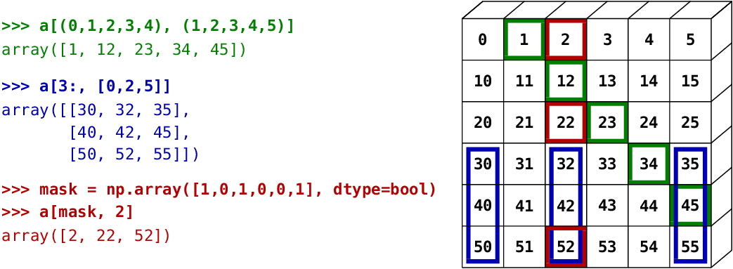
a = np.arange(60).reshape(6, 10)[:,:6]
a
array([[ 0,  1,  2,  3,  4,  5],
       [10, 11, 12, 13, 14, 15],
       [20, 21, 22, 23, 24, 25],
       [30, 31, 32, 33, 34, 35],
       [40, 41, 42, 43, 44, 45],
       [50, 51, 52, 53, 54, 55]])
a[:,2]
array([ 2, 12, 22, 32, 42, 52])
a[:,2:3]
Como resumen (corregir ejemplo rojo!)

Ejercicios
- Dado el array del gráfico (
np.arange(60).reshape(6, 10)[:,:6]):
1.1 Obtener la segunda columna exceptuando el valor de la primera y la última fila
1.2 Obtener toda la submatriz central de 4x4
1.3 "Rodear" el array con ceros (obteniendo una matriz de 8x8)
1.4 Reconfigurar la forma para que cada "fila" resultante se convierta en una matriz de 2x3
- Crear la estructura de datos de un Cubo de Rubik en su estado inicial: 6x3x3 donde cada una de las 6 "caras" i tiene todos sus elementos con valor i
# %load https://gist.githubusercontent.com/mgaitan/1c90f89c49927d329cb6/raw/6d1f1534e8aa692b64e92c4db193500c5a3a2c16/rubik.py
np.zeros([6,3,3]) + np.arange(6)[:,np.newaxis, np.newaxis]
array([[[ 0.,  0.,  0.],
        [ 0.,  0.,  0.],
        [ 0.,  0.,  0.]],

       [[ 1.,  1.,  1.],
        [ 1.,  1.,  1.],
        [ 1.,  1.,  1.]],

       [[ 2.,  2.,  2.],
        [ 2.,  2.,  2.],
        [ 2.,  2.,  2.]],

       [[ 3.,  3.,  3.],
        [ 3.,  3.,  3.],
        [ 3.,  3.,  3.]],

       [[ 4.,  4.,  4.],
        [ 4.,  4.,  4.],
        [ 4.,  4.,  4.]],

       [[ 5.,  5.,  5.],
        [ 5.,  5.,  5.],
        [ 5.,  5.,  5.]]])
np.arange(6)[:, np.newaxis, np.newaxis]
array([[[0]],

       [[1]],

       [[2]],

       [[3]],

       [[4]],

       [[5]]])
c = np.zeros((8,8))
c[1:-1,1:-1] = a
c
array([[  0.,   0.,   0.,   0.,   0.,   0.,   0.,   0.],
       [  0.,   0.,   1.,   2.,   3.,   4.,   5.,   0.],
       [  0.,  10.,  11.,  12.,  13.,  14.,  15.,   0.],
       [  0.,  20.,  21.,  22.,  23.,  24.,  25.,   0.],
       [  0.,  30.,  31.,  32.,  33.,  34.,  35.,   0.],
       [  0.,  40.,  41.,  42.,  43.,  44.,  45.,   0.],
       [  0.,  50.,  51.,  52.,  53.,  54.,  55.,   0.],
       [  0.,   0.,   0.,   0.,   0.,   0.,   0.,   0.]])
a = np.arange(60).reshape(6, 10)[:,:6]

a[0::2,0::2]
np.diag(1+np.arange(4),k=-1)
(tip: investigar la función diag() y rot90()
np.
aleatorio = np.random.normal?
aleatorio = np.random.normal
np.zeros((10,10)) + np.arange(10)
Funciones de reducciones/agregación
numpy tiene muchas funciones y/o métodos de "reducción", que sumarizan información del array. Por ejemplo: sumatoria, media, maximo y minimo, etc.
x = np.array([1, 2, 3, 4])
np.sum(x)
10
Las funciones más importantes también se implementan como métodos
x.sum()
Cuando tenemos un array de más de una dimensión podemos aplicar la función por ejes, a traves del parámetro axis

x = np.array([[1, 1], [2, 2]])
x.sum(axis=1)
array([2, 4])
array([[1, 2],
       [1, 2]])
Funciones de transformación
La función diag poner un array 1D en diagonal (convirtiendolo en 2D) o bien extraer una diagonal de un array 2D dado.
np.diag([1,2,3,4, 4])
array([[1, 0, 0, 0, 0],
       [0, 2, 0, 0, 0],
       [0, 0, 3, 0, 0],
       [0, 0, 0, 4, 0],
       [0, 0, 0, 0, 4]])
Podemos decirle qué diagonal con un offset entero
np.diag([1,2,3], k=-1)
array([[0, 0, 0, 0],
       [1, 0, 0, 0],
       [0, 2, 0, 0],
       [0, 0, 3, 0]])
np.diag(np.arange(30).reshape(5,6))
array([ 0, 7, 14, 21, 28])
rot90 permite rotar un array multidimensional
A
array([[ 0,  1,  2,  3],
       [ 4,  5,  6,  7],
       [ 8,  9, 10, 11]])
np.rot90(A)
array([[ 3,  7, 11],
       [ 2,  6, 10],
       [ 1,  5,  9],
       [ 0,  4,  8]])
np.rot90(A, k=2) # rotamos 180º
array([[11, 10,  9,  8],
       [ 7,  6,  5,  4],
       [ 3,  2,  1,  0]])
Ejercicio
Crear un array 2D de 6x5 de la siguiente forma
array([[0, 0, 0, 0, 5],
       [0, 0, 0, 4, 0],
       [0, 0, 3, 0, 0],
       [0, 2, 0, 0, 0],
       [1, 0, 0, 0, 0],
       [0, 0, 0, 0, 0]])
np.rot90(np.diag(np.arange(1,6), k=1))[:,:-1]
array([[0, 0, 0, 0, 5],
[0, 0, 0, 4, 0],
[0, 0, 3, 0, 0],
[0, 2, 0, 0, 0],
[1, 0, 0, 0, 0],
[0, 0, 0, 0, 0]])
Meshgrids
Una funcion importante es meshgrid, que permite crear una "rejilla" para definir dominios de más de una variable a partir de arrays unidemensionales.
Por ejemplo, si quisieramos definir un dominio de $\R3$ (x,y)
x = np.linspace(0, 10, 11)
y = np.linspace(2, 5, 7)
print(x, y)
grid = Xm, Ym = np.meshgrid(x, y)
print(Xm.shape, Ym.shape)
grid
[  0.   1.   2.   3.   4.   5.   6.   7.   8.   9.  10.] [ 2.   2.5  3.   3.5  4.   4.5  5. ]
(7, 11) (7, 11)
[array([[  0.,   1.,   2.,   3.,   4.,   5.,   6.,   7.,   8.,   9.,  10.],
        [  0.,   1.,   2.,   3.,   4.,   5.,   6.,   7.,   8.,   9.,  10.],
        [  0.,   1.,   2.,   3.,   4.,   5.,   6.,   7.,   8.,   9.,  10.],
        [  0.,   1.,   2.,   3.,   4.,   5.,   6.,   7.,   8.,   9.,  10.],
        [  0.,   1.,   2.,   3.,   4.,   5.,   6.,   7.,   8.,   9.,  10.],
        [  0.,   1.,   2.,   3.,   4.,   5.,   6.,   7.,   8.,   9.,  10.],
        [  0.,   1.,   2.,   3.,   4.,   5.,   6.,   7.,   8.,   9.,  10.]]),
 array([[ 2. ,  2. ,  2. ,  2. ,  2. ,  2. ,  2. ,  2. ,  2. ,  2. ,  2. ],
        [ 2.5,  2.5,  2.5,  2.5,  2.5,  2.5,  2.5,  2.5,  2.5,  2.5,  2.5],
        [ 3. ,  3. ,  3. ,  3. ,  3. ,  3. ,  3. ,  3. ,  3. ,  3. ,  3. ],
        [ 3.5,  3.5,  3.5,  3.5,  3.5,  3.5,  3.5,  3.5,  3.5,  3.5,  3.5],
        [ 4. ,  4. ,  4. ,  4. ,  4. ,  4. ,  4. ,  4. ,  4. ,  4. ,  4. ],
        [ 4.5,  4.5,  4.5,  4.5,  4.5,  4.5,  4.5,  4.5,  4.5,  4.5,  4.5],
        [ 5. ,  5. ,  5. ,  5. ,  5. ,  5. ,  5. ,  5. ,  5. ,  5. ,  5. ]])]

Entonces podemos aplicar una función para este dominio, por ejemplo: $f(x,y) = (xy)^2$
z = (Xm * Ym) ** 2
z
array([[    0.  ,     4.  ,    16.  ,    36.  ,    64.  ,   100.  ,
          144.  ,   196.  ,   256.  ,   324.  ,   400.  ],
       [    0.  ,     6.25,    25.  ,    56.25,   100.  ,   156.25,
          225.  ,   306.25,   400.  ,   506.25,   625.  ],
       [    0.  ,     9.  ,    36.  ,    81.  ,   144.  ,   225.  ,
          324.  ,   441.  ,   576.  ,   729.  ,   900.  ],
       [    0.  ,    12.25,    49.  ,   110.25,   196.  ,   306.25,
          441.  ,   600.25,   784.  ,   992.25,  1225.  ],
       [    0.  ,    16.  ,    64.  ,   144.  ,   256.  ,   400.  ,
          576.  ,   784.  ,  1024.  ,  1296.  ,  1600.  ],
       [    0.  ,    20.25,    81.  ,   182.25,   324.  ,   506.25,
          729.  ,   992.25,  1296.  ,  1640.25,  2025.  ],
       [    0.  ,    25.  ,   100.  ,   225.  ,   400.  ,   625.  ,
          900.  ,  1225.  ,  1600.  ,  2025.  ,  2500.  ]])
y graficamos, por ejemplo, las curvas de nivel
pyplot.contourf(x, y, z)
pyplot.colorbar();

import numpy as np
Ejercicio
- Basado en el ejemplo de wireframe 3D, graficar $z = xe^{-(x^2 + y^2)}$ con $x, y \in [-2, 2]$ con una resolución de 100 puntos en cada eje
x = y = np.linspace(2, -2, 100)
xx,yy = np.meshgrid(x, y)
z = xx*np.exp(-(xx**2 + yy**2))
from mpl_toolkits.mplot3d import axes3d
import matplotlib.pyplot as plt
import numpy as np

fig = plt.figure()
ax = fig.add_subplot(111, projection='3d')
ax.plot_wireframe(xx, yy, z, rstride=10, cstride=10)
---------------------------------------------------------------------------
AttributeError                            Traceback (most recent call last)
<ipython-input-147-ac345543e602> in <module>()
      4
      5 fig = plt.figure()
----> 6 ax = fig.add_subplot(111, projection='3d')
      7 ax.plot_wireframe(xx, yy, z, rstride=10, cstride=10)

/usr/local/lib/python3.4/dist-packages/matplotlib/figure.py in add_subplot(self, *args, **kwargs)
    962                     self._axstack.remove(ax)
    963
--> 964             a = subplot_class_factory(projection_class)(self, *args, **kwargs)
    965
    966         self._axstack.add(key, a)

/usr/local/lib/python3.4/dist-packages/matplotlib/axes/_subplots.py in __init__(self, fig, *args, **kwargs)
     76
     77         # _axes_class is set in the subplot_class_factory
---> 78         self._axes_class.__init__(self, fig, self.figbox, **kwargs)
     79
     80     def __reduce__(self):

/usr/lib/python3/dist-packages/mpl_toolkits/mplot3d/axes3d.py in __init__(self, fig, rect, *args, **kwargs)
     89         Axes.__init__(self, fig, rect,
     90                       frameon=True,
---> 91                       *args, **kwargs)
     92         # Disable drawing of axes by base class
     93         Axes.set_axis_off(self)

/usr/local/lib/python3.4/dist-packages/matplotlib/axes/_base.py in __init__(self, fig, rect, axisbg, frameon, sharex, sharey, label, xscale, yscale, **kwargs)
    435         self._hold = rcParams['axes.hold']
    436         self._connected = {}  # a dict from events to (id, func)
--> 437         self.cla()
    438         # funcs used to format x and y - fall back on major formatters
    439         self.fmt_xdata = None

/usr/lib/python3/dist-packages/mpl_toolkits/mplot3d/axes3d.py in cla(self)
   1043         self._zmargin = 0
   1044
-> 1045         Axes.cla(self)
   1046
   1047         self.grid(rcParams['axes3d.grid'])

/usr/local/lib/python3.4/dist-packages/matplotlib/axes/_base.py in cla(self)
    906         self.containers = []
    907
--> 908         self.grid(self._gridOn, which=rcParams['axes.grid.which'])
    909         props = font_manager.FontProperties(size=rcParams['axes.titlesize'],
    910                                         weight=rcParams['axes.titleweight'])

/usr/lib/python3/dist-packages/mpl_toolkits/mplot3d/axes3d.py in grid(self, b, **kwargs)
   1254         if len(kwargs) :
   1255             b = True
-> 1256         self._draw_grid = maxes._string_to_bool(b)
   1257
   1258     def ticklabel_format(self, **kwargs) :

AttributeError: 'module' object has no attribute '_string_to_bool'
<matplotlib.figure.Figure at 0x7fa2d4869320>
Fancy indexing y máscaras
Numpy permite indizar a través de una secuencia
a = np.random.random_integers(0, 30, 10)   # 10 enteros aleatorios entre [0, 30]
a
array([21, 27, 2, 27, 17, 7, 3, 5, 15, 7])
Esto se conoce como fancy indexing
a[[1, 2, 4, 1]] # selecciona el elemento 1, 2, el 4 y de nuevo el 1
array([27, 2, 17, 27])
Por otro lado, podemos indexar elementos a traves de un array (o cualquier secuencia array-like) de tipo booleano. Esto es, hacer una máscara
a[np.array([True, False, True, True, False, False, True, False, False])]
array([21, 2, 27, 3])
Pero por otro lado sabemos que via broadcasting podemos obtener un array booleano
a > 15 # qué elementos de a son mayores a 10 ?
array([ True, True, False, True, True, False, False, False, False, False], dtype=bool)
Por lo tanto, podemos "filtrar" los valores que cumplan determinada condición en un array
a[a > 10]
array([21, 27, 27, 17, 15])
Más aun, podemos combinar condiciones a través de operadores lógicos
a[(a > 10) & (a < 25)]
array([21, 17, 15])
(Este tipo de slicing especial crea copias, no vistas. Usar cuando lo amerite.)
Si en vez de los valores que cumplen una condición, queremos las posiciones, podemos usar la función where
np.where(a > 15) # devuelve las posiciones.
Además, la función where funciona como estructura ternaria a nivel arrays
b = 0
# para cada i-elemento a[i] si True, si no b[i] (o constante)
np.where(a > 10, a, b)
array([21, 27, 0, 27, 17, 0, 0, 0, 15, 0])
Ejemplos
Lectura desde texto y archivos
Como numpy se especializa en manejar números, tiene muchas funciones para crear arrays a partir de información numérica a partir de texto o archivos (como los CSV, por ejemplo).
a_desde_str = np.fromstring("""1.0 2.3   3.0 4.1
-3.1 2  5.0 4.5""", sep=" ", dtype=float)
a_desde_str.shape = (2, 4)
a_desde_str
array([[ 1. ,  2.3,  3. ,  4.1],
       [-3.1,  2. ,  5. ,  4.5]])
Para cargar desde un archivo existe la función loadtxt. Por ejemplo tenemos el archivo data/critical.dat que es el resultado del cálculo de una linea crítica global para un sistema químico binario.
!head data/critical.dat
T(K)     P(bar)   d(mol/L)   x(1)
 CRI
 304.2100   73.8300    8.7568  0.000000 0.10000E+01
 304.2056   73.8318    8.7570  0.000050 0.99995E+00   3   1
 304.2011   73.8340    8.7572  0.000117 0.99988E+00   2   1
 304.1920   73.8384    8.7577  0.000250 0.99975E+00   2   1
 304.1740   73.8472    8.7586  0.000517 0.99948E+00   2   1
 304.1379   73.8649    8.7604  0.001050 0.99895E+00   2   1
 304.0657   73.9002    8.7640  0.002117 0.99788E+00   2   1
 303.9211   73.9706    8.7711  0.004250 0.99575E+00   2   1
np.loadtxt?
Vemos que el patrón es en columnas separadas por espacios en blanco y las dos primeras filas son headers
cri_data = np.loadtxt('data/critical.dat', skiprows=2, usecols=[0, 1, 2, 3])
cri_data.shape
(211, 4)
Por defecto, devuelve una matriz 2D numero_lineas x columnas, o sea, la fila 0 es la primer linea de números
cri_data[:, 0]
array([ 304.21  ,  304.2056,  304.2011,  304.192 ,  304.174 ,  304.1379,
        304.0657,  303.9211,  303.6309,  303.2894,  302.9461,  302.6013,
        302.2547,  301.9064,  301.5565,  301.2048,  300.8514,  300.4962,
        300.1394,  299.7807,  299.4203,  299.0581,  298.6941,  298.3283,
        297.9606,  297.5911,  297.2198,  296.8466,  296.4716,  296.0946,
        295.7158,  295.335 ,  294.9524,  294.5677,  294.1812,  293.7927,
        293.4022,  293.0097,  292.6152,  292.2187,  291.8201,  291.4195,
        291.0169,  290.6122,  290.2054,  289.7965,  289.3855,  288.9724,
        288.5572,  288.1398,  287.7202,  287.2984,  286.8745,  286.4484,
        286.02  ,  285.5894,  285.1566,  284.7215,  284.2841,  283.8444,
        283.4025,  282.9582,  282.5116,  282.0627,  281.6114,  281.1577,
        280.7017,  280.2432,  279.7824,  279.3192,  278.8535,  278.3854,
        277.9148,  277.4417,  276.9662,  276.4882,  276.0077,  275.5246,
        275.0391,  274.551 ,  274.0603,  273.5671,  273.0714,  272.573 ,
        272.0721,  271.5686,  271.0625,  270.5537,  270.0424,  269.5284,
        269.0117,  268.4925,  267.9705,  267.446 ,  266.9187,  266.3888,
        265.8562,  265.321 ,  264.7831,  264.2425,  263.6992,  263.1532,
        262.6045,  262.0532,  261.4991,  260.9424,  260.383 ,  259.821 ,
        259.2562,  258.6888,  258.1187,  257.546 ,  256.9706,  256.3925,
        255.8118,  255.2285,  254.6426,  254.0541,  253.4629,  252.8692,
        252.2729,  251.6741,  251.0727,  250.4688,  249.8625,  249.2536,
        248.6422,  248.0284,  247.4122,  246.7935,  246.1725,  245.5491,
        244.9234,  244.2953,  243.665 ,  243.0323,  242.3974,  241.7603,
        241.121 ,  240.4795,  239.8358,  239.19  ,  238.542 ,  237.892 ,
        237.2398,  236.5856,  235.9294,  235.2711,  234.6108,  233.9484,
        233.2841,  232.6178,  231.9494,  231.2791,  230.6067,  229.9324,
        229.256 ,  228.5776,  227.8971,  227.2145,  226.5299,  225.843 ,
        225.154 ,  224.4628,  223.7692,  223.0734,  222.3751,  221.6743,
        220.971 ,  220.265 ,  219.5564,  218.8448,  218.1304,  217.4129,
        216.6923,  215.9683,  215.2409,  214.51  ,  213.7753,  213.0367,
        212.2941,  211.5473,  210.7961,  210.0403,  209.2797,  208.5141,
        207.7433,  206.967 ,  206.1851,  205.3974,  204.6034,  203.8032,
        202.9963,  202.1825,  201.3615,  200.5331,  199.697 ,  198.8528,
        198.0004,  197.1393,  196.2693,  195.3901,  194.5014,  193.6027,
        192.6939,  191.7744,  190.8441,  190.7051,  190.6356,  190.6008,
        190.564 ])
Si directamente queremos los vectores (las columnas), podemos pedir que "desempaque" las columnas
t, p, d, x = np.loadtxt('data/critical.dat', skiprows=2, usecols=[0, 1, 2, 3], unpack=True) # o loadtxt().T
t
t.size
Podemos graficar algo sencillo
%matplotlib inline
from matplotlib import pyplot
pyplot.plot(, p, 'r')   # el tercer parámetro es el formato
pyplot.title('Critical pressure vs temperature')
pyplot.grid()
pyplot.xlabel('Temperature [K]')
pyplot.ylabel('Pressure [bar]')
# el punto y coma evita el output
pyplot.show();

Otras herramientas de numpy
ya mencionamos el subpaquete numpy.random que tiene funciones análogas a random de la biblioteca estándar, pero que construyen arrays
Otras funciones y utilidades incorporadas en numpy
## tanto trabajo con nuestra función "baskara" y ya estaba hecho!
np.roots([2, 2, 1j])
array([-1.13600982+0.39307569j, 0.13600982-0.39307569j])
# encima funciona para grado n
np.roots([1j, -4+0.4j, 18, -np.pi, 0])  # polinomio de grado 5!
De manera contraria, la función poly devuelve los coeficientes de un polinomio dadas sus raíces
np.poly([-2, 2, 1j])
array([ 1.+0.j, 0.-1.j, -4.+0.j, 0.+4.j])
np.poly(np.array([-1.13600982+0.39307569j, 0.13600982-0.39307569j]))
array([ 1.00000000e+00+0.j , 1.00000000e+00+0.j , 6.93254368e-09+0.5j])
También podemos encontrar la inversa de una matriz
A = np.array([[1,2],[3,4]])
invA = np.linalg.inv(A)
invA
array([[-2. ,  1. ],
       [ 1.5, -0.5]])
y calcular el producto punto
np.dot(A,invA) # equivalente A @ invA en py3.5
array([[  1.00000000e+00,   1.11022302e-16],
       [  0.00000000e+00,   1.00000000e+00]])
que son las operaciones para resolver un sistema de ecuaciones lineales $Ax = b$
A = np.array([[1, 2], [0.5, -2]])
b = np.array([4, 5.2])

x = np.linalg.solve(A, b)
x
array([ 6.13333333, -1.06666667])
Ejercicios
- Graficar el polinomio con raices en -4., 2. y -1. entre [-5, 3]
Resuelva el siguiente sistema de ecuaciones
$$\begin{array} - -x + z = -2\\ 2x - y + z = 1 \\ -3x + 2y -2z = -1 \end{array}$$
Matplolib orientado a objeto
Hasta ahora hemos usado pyplot, el módulo de matptlotlib que emula la forma de uso (la API) de Matlab. En este modo cada función que invocamos afecta un estado interno en el que podemos ir "acumulando" cambios (por ejemplo, el título, la etiqueta de los ejes, etc)
Este tipo de funcionamiento es práctico y fácil, pero limitado, porque es totalmente "lineal" (procedural) . Para mejorar las prestaciones y la posibilidad de "tocar" todo lo que queramos, tenemos que usar el modo "orientado a objetos". Este modo es un poco más verborrágico pero también más explícito y potente. En general se usa una mezcla entre la "practicidad" de pyplot (modo procedural) y la orientación a objetos. Veamos un ejemplo
from matplotlib import pyplot as plt
t = x = np.arange(0, 10, 0.1)
y = np.random.randn(t.size)

fig = plt.figure()      # con una funcion de pyplot creamos un objeto tipo Figure.
print(type(fig))
ax = fig.add_subplot(1, 1, 1)  # en la posicion 1-1 creamos un Subplot en nuestro objeto fig (que tendrá solo un plot)
print(type(ax))
lines = ax.plot(t, y)      # en ese objeto plot graficamos x vs y
print(type(lines))
t = ax.set_title('random numbers')    # y al mismo plot le ponemos un titulo
print(type(t))
plt.show()    # por ultimo mostramos el grafico
<class 'matplotlib.figure.Figure'>
<class 'matplotlib.axes._subplots.AxesSubplot'>
<class 'list'>
<class 'matplotlib.text.Text'>

Supongamos que queremos graficar muchas curvas en el mismo Subplot.
fig = plt.figure()      # con una funcion de pyplot creamos un objeto tipo Figure.
ax = fig.add_subplot(1, 1, 1)  # en la posicion 1-1 creamos un Subplot en nuestro objeto fig (que tendrá solo un plot)


ax.plot(x, x + 1, c='red', label=r'$y = x + 1$' )        # label usando LaTex
ax.plot(x, .5*x - 2, c='green', label=r'$y = 0.5x - 2$' )
ax.plot(x, -x, c='black', label=r'$y = -x$' )
ax.grid()
ax.legend(loc="upper left")
plt.show()

Pero también podemos tener una figura con múltiples subplots
x = np.linspace(0, 2*np.pi, 100)
fig = plt.figure()
ax1 = fig.add_subplot(2, 1, 1)    # el plot 1 en una figura de 2x1
ax1.set_title('Seno')
ax1.plot(x, np.sin(x), c='red')
ax2 = fig.add_subplot(2, 1, 2)   # el plot 2 en una figura de 2x1
ax2.plot(x, np.cos(x), c='blue')
ax2.set_title('Coseno')
fig.tight_layout()  # ajusta el espaciado entre los subplots
plt.show()

Aunque ya la mostramos, todavia tenemos control sobre los objetos. Por ejemplo, podemos guardar la figura en un archivo
fig.savefig('senos.png', format='png')
!eog senos.png
Otra manera de crear figuras con múltiples subplots es usar la función subplots. Por supuesto, cada gráfico puede ser de un tipo distinto
from matplotlib import pyplot as plt
import numpy as np

xx = np.linspace(-0.75, 1., 100)
n = np.arange(0,6)

# devuelve la figura y la lista de subplots
fig, axes = plt.subplots(1, 5, figsize=(17,3))

# scatter grafica puntos pero no los une
axes[0].scatter(xx, xx + 0.25, c='red', marker='^')

axes[1].step(n, n**2, 'g', lw=2)

axes[2].bar(n, n**2, align="center", width=0.5, alpha=0.5)

axes[3].fill_between(x, x**2, x**3, color="green", alpha=0.5);

# ax = fig.add_subplot(1, 5, 5, projection='3d')
# t = np.linspace(0, 2 *np.pi, 100)
# ax.plot(t, t, t, color='blue', lw=3)
pyplot.show()

Gráficos 3D
Hacer gráficos en 3D no es el fin principal de matplotlib y por eso está en un toolkit aparte, pero es muy fácil. Primero hace falta importar la clase para el tipo Axes3D
from mpl_toolkits.mplot3d.axes3d import Axes3D
Eso "parcha" la clase para que los subplot acepte la proyección 3D
fig = plt.figure(figsize=(10,8))

# `ax` is a 3D-aware axis instance, because of the projection='3d' keyword argument to add_subplot
ax = fig.add_subplot(1, 1, 1, projection='3d')

theta = np.linspace(-4 * np.pi, 4 * np.pi, 1000)
z = np.linspace(-2, 2, 1000)
r = z**2 + 1
x = r * np.sin(theta)
y = r * np.cos(theta)
ax.plot(x,y,z, lw=1.5)
plt.show()
---------------------------------------------------------------------------
AttributeError                            Traceback (most recent call last)
<ipython-input-179-e6691d232c9a> in <module>()
      2
      3 # `ax` is a 3D-aware axis instance, because of the projection='3d' keyword argument to add_subplot
----> 4 ax = fig.add_subplot(1, 1, 1, projection='3d')
      5
      6 theta = np.linspace(-4 * np.pi, 4 * np.pi, 1000)

/usr/local/lib/python3.4/dist-packages/matplotlib/figure.py in add_subplot(self, *args, **kwargs)
    962                     self._axstack.remove(ax)
    963
--> 964             a = subplot_class_factory(projection_class)(self, *args, **kwargs)
    965
    966         self._axstack.add(key, a)

/usr/local/lib/python3.4/dist-packages/matplotlib/axes/_subplots.py in __init__(self, fig, *args, **kwargs)
     76
     77         # _axes_class is set in the subplot_class_factory
---> 78         self._axes_class.__init__(self, fig, self.figbox, **kwargs)
     79
     80     def __reduce__(self):

/usr/lib/python3/dist-packages/mpl_toolkits/mplot3d/axes3d.py in __init__(self, fig, rect, *args, **kwargs)
     89         Axes.__init__(self, fig, rect,
     90                       frameon=True,
---> 91                       *args, **kwargs)
     92         # Disable drawing of axes by base class
     93         Axes.set_axis_off(self)

/usr/local/lib/python3.4/dist-packages/matplotlib/axes/_base.py in __init__(self, fig, rect, axisbg, frameon, sharex, sharey, label, xscale, yscale, **kwargs)
    435         self._hold = rcParams['axes.hold']
    436         self._connected = {}  # a dict from events to (id, func)
--> 437         self.cla()
    438         # funcs used to format x and y - fall back on major formatters
    439         self.fmt_xdata = None

/usr/lib/python3/dist-packages/mpl_toolkits/mplot3d/axes3d.py in cla(self)
   1043         self._zmargin = 0
   1044
-> 1045         Axes.cla(self)
   1046
   1047         self.grid(rcParams['axes3d.grid'])

/usr/local/lib/python3.4/dist-packages/matplotlib/axes/_base.py in cla(self)
    906         self.containers = []
    907
--> 908         self.grid(self._gridOn, which=rcParams['axes.grid.which'])
    909         props = font_manager.FontProperties(size=rcParams['axes.titlesize'],
    910                                         weight=rcParams['axes.titleweight'])

/usr/lib/python3/dist-packages/mpl_toolkits/mplot3d/axes3d.py in grid(self, b, **kwargs)
   1254         if len(kwargs) :
   1255             b = True
-> 1256         self._draw_grid = maxes._string_to_bool(b)
   1257
   1258     def ticklabel_format(self, **kwargs) :

AttributeError: 'module' object has no attribute '_string_to_bool'
<matplotlib.figure.Figure at 0x7fa2d45b40b8>
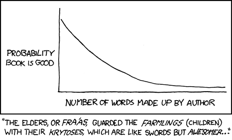
¡Matplotlib es genial! Es libre y gratis y brinda resultados excepcionales. Seguro lo usarás para tu próximo paper/poster


import antigravity
Muchas veces, la tira tiene gráficos de este estilo
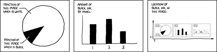

Si intentáramos hacer nuestra propia versión, arruinaríamos el chiste
%matplotlib inline
from matplotlib import pyplot as plt
import numpy as np

fig = plt.figure()
ax = fig.add_subplot(1, 1, 1)
ax.bar([-0.125, 1.0-0.125], [0, 100], 0.25)
ax.spines['right'].set_color('none')
ax.spines['top'].set_color('none')
ax.xaxis.set_ticks_position('bottom')
ax.set_xticks([0, 1])
ax.set_xlim([-0.5, 1.5])
ax.set_ylim([0, 110])
ax.set_xticklabels(['CONFIRMED BY\nEXPERIMENT', 'REFUTED BY\nEXPERIMENT'])
plt.yticks([])
plt.title("CLAIMS OF SUPERNATURAL POWERS");

¿Pero qué tal usar el modo XKCD de Matplotlib?
with plt.xkcd():
    fig = plt.figure()
    ax = fig.add_subplot(1, 1, 1)
    ax.bar([-0.125, 1.0-0.125], [0, 100], 0.25)
    ax.spines['right'].set_color('none')
    ax.spines['top'].set_color('none')
    ax.xaxis.set_ticks_position('bottom')
    ax.set_xticks([0, 1])
    ax.set_xlim([-0.5, 1.5])
    ax.set_ylim([0, 110])
    ax.set_xticklabels(['CONFIRMED BY\nEXPERIMENT', 'REFUTED BY\nEXPERIMENT'])
    plt.yticks([])
    plt.title("CLAIMS OF SUPERNATURAL POWERS")

with plt.xkcd():
    labels = 'Frogs', 'Hogs', 'Dogs', 'Logs'
    sizes = [15, 30, 45, 10]
    colors = ['yellowgreen', 'gold', 'lightskyblue', 'lightcoral']
    explode = (0, 0.1, 0, 0) # only "explode" the 2nd slice (i.e. 'Hogs')

    plt.pie(sizes, explode=explode, labels=labels, colors=colors,
            autopct='%1.f%%', shadow=True, startangle=60)
    # Set aspect ratio to be equal so that pie is drawn as a circle.
    plt.axis('equal');

Cualquier gráfico se puede "xkcdear" ;-). http://matplotlib.org/xkcd/