A brief introduction to JuliaReach
Marcelo Forets, Universidad de la República, Uruguay.
Berlin Julia Users Meetup 2019, Berlin, August 7th, 2019
Outline of this talk
Context of the JuliaReach org
LazySets: from low dimensions to high dimensions using multiple dispatch
Applications
- Neural network verification
- Reachability analysis of uncertain dynamical systems
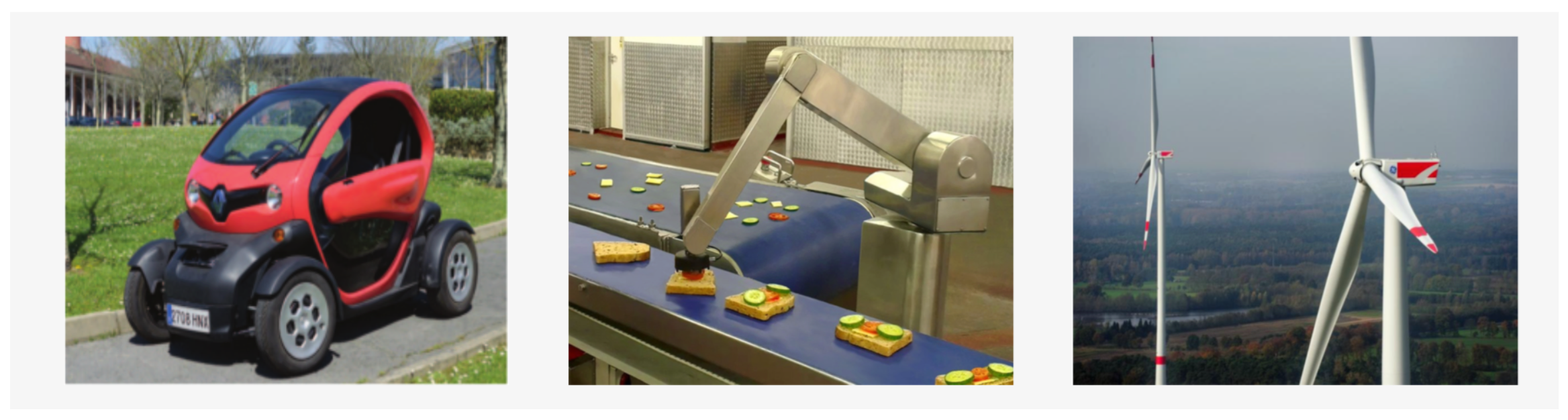
In particular we focus on cyber-physical systems: a device that by means of computation is able to control or interact with a physical process
Examples:
- embedded controllers (aircrafts, autonomous cars, ...)
- medical devices; safety-critical or mission-critical devices; power systems stability; ...
Who makes JuliaReach?

Bogomolov, S., Forets, M., Frehse, G., Potomkin, K., & Schilling, C. (2019, April). JuliaReach: a toolbox for set-based reachability. In Proceedings of the 22nd ACM International Conference on Hybrid Systems: Computation and Control (pp. 39-44), ACM.
An intro to LazySets
using LazySets, Plots
using AbstractTrees

AbstractTrees.children(x::Type) = subtypes(x)
print_tree(LazySet)
Convex sets

Balls

More balls

Unbounded sets

Translation
![]()
Minkowski sum

Linear map

Projection

Union (not convex)

Convex hull

Intersection

A high-dimensional demo
- We'l work with a 100-dimensional set which has...
exp(100 * log(2)) ≈ 1.2676506002282317e30vertices.
H = rand(Hyperrectangle, dim=100);
d = ones(Float64, 100);
@btime σ($d, $H);
σ(d, H) ∈ H
M = rand(100, 100)
P = project(M * H, [99, 100], LinearMap);
@btime project($M * $H, [99, 100], LinearMap);
plot(overapproximate(P, HPolygon, 1e-2))
@btime overapproximate($P, HPolygon, 1e-2)
f(B) = M * H ⊕ B
B = Ball2(100 * rand(100), 2.0)
P = project(f(B), [99, 100], LinearMap);
@btime f($B)
plot!(overapproximate(P, HPolygon, 1e-3))
@btime overapproximate($P, HPolygon, 1e-3)
Fair enough, show me the trick.

[KAR19] Stefan Karpinksi (Julia Computing). The Unreasonable Effectiveness of Multiple Dispatch. JuliaCon 2019
The lazy evaluation paradigm
- Principle of lazy evaluation: delay the evaluation of an expression until its value is needed.
- Question: what do i really need to compute if i just want $\rho(d, MH \oplus B)$?
- Answer: combine basic machinery in convex geometry with the lazy evaluation paradigm, letting Julia to handle the appropriate dispatch for your computation.
Calculus with suport functions

Calculus with suport functions (cont.)

Case study: lazy Minkowski sum
- Implement the Minkowski sum operator as a new
LazySet, with two basic functions:- dimension
- compute its support vector (or support function)
function ρ(d::AbstractVector{N}, ms::MinkowskiSum{N}) where {N<:Real}
    return ρ(d, ms.X) + ρ(d, ms.Y)
end
Hold on, did he just say that ⊕ is a set?
struct MinkowskiSum{N<:Real, S1<:LazySet{N}, S2<:LazySet{N}} <: LazySet{N}
    X::S1
    Y::S2

    # default constructor with dimension check
    function MinkowskiSum{N, S1, S2}(X::S1, Y::S2) where
            {N<:Real, S1<:LazySet{N}, S2<:LazySet{N}}
        @assert dim(X) == dim(Y) "sets in a Minkowski sum must have the " *
            "same dimension"
        return new{N, S1, S2}(X, Y)
    end
end
@neutral(MinkowskiSum, ZeroSet)
@absorbing(MinkowskiSum, EmptySet)
⊕(X::LazySet, Y::LazySet) = MinkowskiSum(X, Y)
Reachability Analysis in JuliaReach
The problem
- Complex, real-world systems are prone to failures
- New industrial standars explicitly recommend the user of formal methods: DO-178C (avionics), ISO 26262 (automotive systems), IEC 62304 (medical devices), and CENELEC EN 50128 (railway systems).

- Engineers need safety and reliability guarantees to take design decisions under non-deterministic inputs, parameters or noise
$\Longrightarrow$ The field of reachability analysis is concerned with understanding the set of all possible behaviors of such systems.
Bogomolov, S., Forets, M., Frehse, G., Potomkin, K., & Schilling, C. (2019, April). JuliaReach: a toolbox for set-based reachability. In Proceedings of the 22nd ACM International Conference on Hybrid Systems: Computation and Control (pp. 39-44), ACM.
References to our research work
[BFFPSV18] Reach Set Approximation through Decomposition with Low-dimensional Sets and High-dimensional Matrices. S. Bogomolov, M. Forets, G. Frehse, , A. Podelski, C. Schilling and F. Viry (2018) HSCC'18 Proceedings of the 21st International Conference on Hybrid Systems: Computation and Control: 41–50.
[ARCH-COMP18-AFF] ARCH-COMP18 Category Report: Continuous and Hybrid Systems with Linear Continuous Dynamics. M. Althoff, S. Bak, X. Chen, C. Fan, M. Forets, G. Frehse, N. Kochdumper, Y. Li, S. Mitra, R. Ray, C. Schilling and S. Schupp (2018) ARCH18. 5th International Workshop on Applied Verification of Continuous and Hybrid Systems, 54: 23–52. doi: 10.29007/73mb.
[BFFPS19] JuliaReach: a Toolbox for Set-Based Reachability. Sergiy Bogomolov, Marcelo Forets, Goran Frehse, Kostiantyn Potomkin, Christian Schilling. Published in Proceedings of HSCC'19: 22nd ACM International Conference on Hybrid Systems: Computation and Control (HSCC'19).
References to our research work (cont.)
[BFFPS19b] Reachability analysis of linear hybrid systems via block decomposition. Sergiy Bogomolov, Marcelo Forets, Goran Frehse, Kostiantyn Potomkin, Christian Schilling.
[ARCH-COMP19-AFF] ARCH-COMP19 Category Report: Continuous and Hybrid Systems with Linear Continuous Dynamics. Matthias Althoff, Stanley Bak, Marcelo Forets, Goran Frehse, Niklas Kochdumper, Rajarshi Ray, Christian Schilling and Stefan Schupp (2019) ARCH19. 6th International Workshop on Applied Verification of Continuous and Hybrid Systems, vol 61, pages 14–40 doi: 10.29007/bj1w.
[ARCH-COMP19-NLN] ARCH-COMP19 Category Report: Continuous and Hybrid Systems with Nonlinear Dynamics. Fabian Immler, Matthias Althoff, Luis Benet, Alexandre Chapoutot, Xin Chen, Marcelo Forets, Luca Geretti, Niklas Kochdumper, David P. Sanders and Christian Schilling (2019) ARCH19. 6th International Workshop on Applied Verification of Continuous and Hybrid Systems, vol 61, pages 41–61 doi: 10.29007/bj1w.
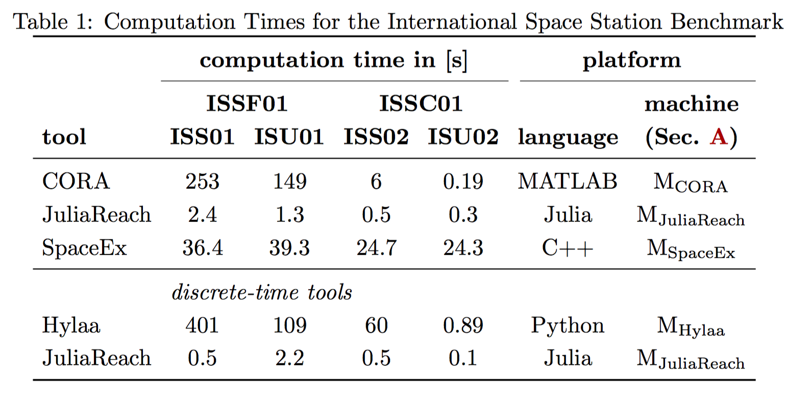
ISS Benchmark
- ISS: structural model of component 1R (Russian service module) of the international space station
- 270 state variables with three uncertain inputs
- linear time-invariant: $x'(t) = Ax(t) + Bu(t)$, $u(t) \in \mathcal{U}$, $y(t) = Cx(t) + Du(t)$
- specification: output $y_3(t)$ is within the range $[0.0007, 0.0007]$ for all $t \in [0, 20]$.

ISS Benchmark

ISS Benchmark

ISS Benchmark
Quadrotor benchmark
- nonlinear
- 12 dimensions
- safety property: stabilization of the height after some given time horizon, which should stay within given bounds
- uncertain positions and uncertain velocities

Quadrotor benchmark

Quadrotor benchmark

Quadrotor benchmark

Quadrotor benchmark

Verifying Deep Neural Networks

- Deep neural networks are widely used for nonlinear function approximation with applications ranging from computer vision to control.
- It can be very challenging to verify whether a particular network satis es certain input-output properties.
LazySetsis being used in https://github.com/sisl/NeuralVerification.jl as a convenient framework to work with sets- (work-in-progress) We can scale even further, using lazy intersections and lazy
ReLUfunctions (it's a bit rough, but if you are curious, see my notebook https://nbviewer.jupyter.org/github/mforets/escritoire/blob/master/reachability/Lazy_NNets.ipynb)
If you are interested check https://github.com/sisl/NeuralVerification.jl and their recent review paper:

Any sufficiently advanced technology is indistinguishable from magic.
(Clark's third law)
Conclusions
- Convex sets are expressive, calculus is tractable.
- Closure under most standard set operations.
- Support functions allow for lazy (on-demand) computations.
- Non-convex sets: approximate by (union of) convex sets.
- Julia is an excellent choice to reason about set-based algorithms.
Acknowledgements
JuliaReach development is led by:
- Marcelo Forets (Univ. de la República, Uruguay)
- Christian Schilling (Institute of Science and Technology, Austria)
Contributors to JuliaReach open projects include:
- A. Deshmuhk (Indian Institute of Information Technology, India)
- B. Garate (Univ. de la República, Uruguay)
- S. Guadalupe (Univ. de la República, Uruguay)
- N. Kekatos (Univ. Grenoble Alpes, France)
- B. Legat (UCLouvain, Belgium)
- K. Potomkin (ANU, Australia)
- A. Rocca (INRIA, France)
- F. Viry (CERFACS, France)
Scientific collaborators:
- L. Benet (UNAM, México)
- S. Bogomolov (ANU, Australia)
- G. Frehse (ENSTA ParisTech, France)
- A. Podelski (Univ. of Freiburg, Germany),
- David P. Sanders (UNAM, México) </font>
Join the effort! https://github.com/juliareach
<https://gitter.im/JuliaReach/Lobby
Contact: mforets@gmail.com http://github.com/mforets