| What? | Relevant classes and/or methods |
|---|---|
| Finding model and observation data | pya.browse_database |
| Reading of *gridded* model data | pya.io.ReadGridded |
| Working with *gridded* data | pya.GriddedData |
| Reading of *ungridded* observation data | pya.io.ReadUngridded |
| Working with *ungridded* data | pya.UngriddedData |
| Working with data from individual site locations | pya.StationData |
| Colocation of model and observational data | High-level: pya.colocation_auto |
Low-level: pya.colocation |
|
| Working with colocated data | pya.ColocatedData |
In a graphical way it introduces the main data object and processing routines for model and observation comparisons with pyaerocom, illustrated in the following flowchart:
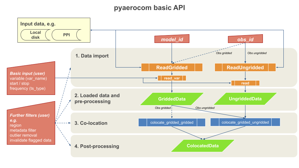
Only that in this example "Data server" is the local computer that has the minimal testdataset as an example dataset.
import pyaerocom as pya
pya.__version__
/home/jonasg/miniconda3/envs/pyadev/lib/python3.9/site-packages/geonum/__init__.py:26: UserWarning: Plotting of maps etc. is deactivated, please install Basemap
  warn('Plotting of maps etc. is deactivated, please install Basemap')
'0.12.0.dev1'
Should be at least 0.10.X
Check access to testdata
NOTE: details regarding testdata access and intialization are covered in tutorial notebook getting_started_setup.ipynb.
from pyaerocom.testdata_access import initialise
initialise()
Adding data search directory /home/jonasg/MyPyaerocom/testdata-minimal/modeldata.
Adding data search directory /home/jonasg/MyPyaerocom/testdata-minimal/obsdata.
Adding data search directory /home/jonasg/MyPyaerocom/testdata-minimal/config.
Adding ungridded dataset AeronetSunV3L2Subset.daily located at /home/jonasg/MyPyaerocom/testdata-minimal/obsdata/AeronetSunV3Lev2.daily/renamed.Reader: <class 'pyaerocom.io.read_aeronet_sunv3.ReadAeronetSunV3'>
Adding ungridded dataset AeronetSDAV3L2Subset.daily located at /home/jonasg/MyPyaerocom/testdata-minimal/obsdata/AeronetSDAV3Lev2.daily/renamed.Reader: <class 'pyaerocom.io.read_aeronet_sdav3.ReadAeronetSdaV3'>
Adding ungridded dataset AeronetInvV3L2Subset.daily located at /home/jonasg/MyPyaerocom/testdata-minimal/obsdata/AeronetInvV3Lev2.daily/renamed.Reader: <class 'pyaerocom.io.read_aeronet_invv3.ReadAeronetInvV3'>
Adding ungridded dataset EBASSubset located at /home/jonasg/MyPyaerocom/testdata-minimal/obsdata/EBASMultiColumn.Reader: <class 'pyaerocom.io.read_ebas.ReadEbas'>
Adding ungridded dataset AirNowSubset located at /home/jonasg/MyPyaerocom/testdata-minimal/obsdata/AirNowSubset.Reader: <class 'pyaerocom.io.read_airnow.ReadAirNow'>
Adding ungridded dataset G.EEA.daily.Subset located at /home/jonasg/MyPyaerocom/testdata-minimal/obsdata/GHOST/data/EEA_AQ_eReporting/daily.Reader: <class 'pyaerocom.io.read_ghost.ReadGhost'>
Adding ungridded dataset G.EEA.hourly.Subset located at /home/jonasg/MyPyaerocom/testdata-minimal/obsdata/GHOST/data/EEA_AQ_eReporting/hourly.Reader: <class 'pyaerocom.io.read_ghost.ReadGhost'>
Adding ungridded dataset G.EBAS.daily.Subset located at /home/jonasg/MyPyaerocom/testdata-minimal/obsdata/GHOST/data/EBAS/daily.Reader: <class 'pyaerocom.io.read_ghost.ReadGhost'>
Adding ungridded dataset G.EBAS.hourly.Subset located at /home/jonasg/MyPyaerocom/testdata-minimal/obsdata/GHOST/data/EBAS/hourly.Reader: <class 'pyaerocom.io.read_ghost.ReadGhost'>
pyaerocom-testdata is ready to be used. The data is available at /home/jonasg/MyPyaerocom/testdata-minimal
Model data: Reading of and working with gridded data
This section provides an introduction into the following pyaerocom classes and architectures:
*you may click the links to see the online documentation of these classes.
Pre-remark on the ReadGridded class
As you could see in tutorial getting_started_setup.ipynb the ReadGridded class makes extensive use of the AeroCom file naming conventions. So if you have model data that is stored using different conventions (e.g. CMIP6), this class will not be of much help (yet) for filtering the correct files to read. In that case you may locate a model NetCDF file yourself and pass it directly into a GriddedData object on initialisation.
Find model data
The testdataset contains data from the TM5 model, which is used in the following. You can use the browse_database function of pyaerocom to find model ID's (which can be quite cryptic sometimes) using wildcard pattern search.
pya.browse_database('*TM5*')
Pyaerocom ReadGridded
---------------------
Data ID: TM5JRCCY2IPCCV1_SR6SA
Data directory: /lustre/storeA/project/aerocom/aerocom-users-database/HTAP-PHASE-I/TM5JRCCY2IPCCV1_SR6SA/renamed
Available experiments: ['SR6SA']
Available years: [2001]
Available frequencies ['monthly']
Available variables: ['MMR_BCSR6SA', 'MMR_NO3SR6SA', 'MMR_POMSR6SA', 'MMR_SO4SR6SA']

Pyaerocom ReadGridded
---------------------
Data ID: TM5JRCCY2IPCCV1_SR6NA
Data directory: /lustre/storeA/project/aerocom/aerocom-users-database/HTAP-PHASE-I/TM5JRCCY2IPCCV1_SR6NA/renamed
Available experiments: ['SR6NA']
Available years: [2001]
Available frequencies ['monthly']
Available variables: ['MMR_BCSR6NA', 'MMR_NO3SR6NA', 'MMR_POMSR6NA', 'MMR_SO4SR6NA']

Pyaerocom ReadGridded
---------------------
Data ID: TM5-JRC-cy2-ipcc-v1_SR1
Data directory: /lustre/storeA/project/aerocom/aerocom-users-database/HTAP-PHASE-I/TM5-JRC-cy2-ipcc-v1_SR1/renamed
Available experiments: ['SR1']
Available years: [2001]
Available frequencies ['monthly']
Available variables: ['vmro3']

Pyaerocom ReadGridded
---------------------
Data ID: TM5JRCCY2IPCCV1_SR6EU
Data directory: /lustre/storeA/project/aerocom/aerocom-users-database/HTAP-PHASE-I/TM5JRCCY2IPCCV1_SR6EU/renamed
Available experiments: ['SR6EU']
Available years: [2001]
Available frequencies ['monthly']
Available variables: ['MMR_BCSR6EU', 'MMR_NO3SR6EU', 'MMR_POMSR6EU', 'MMR_SO4SR6EU']

Pyaerocom ReadGridded
---------------------
Data ID: TM5JRCCY2IPCCV1_SR6EA
Data directory: /lustre/storeA/project/aerocom/aerocom-users-database/HTAP-PHASE-I/TM5JRCCY2IPCCV1_SR6EA/renamed
Available experiments: ['SR6EA']
Available years: [2001]
Available frequencies ['monthly']
Available variables: ['MMR_BCSR6EA', 'MMR_NO3SR6EA', 'MMR_POMSR6EA', 'MMR_SO4SR6EA']

Pyaerocom ReadGridded
---------------------
Data ID: TM5JRCCY2IPCCV1_SR1
Data directory: /lustre/storeA/project/aerocom/aerocom-users-database/HTAP-PHASE-I/TM5JRCCY2IPCCV1_SR1/renamed
Available experiments: ['SR1']
Available years: [2001]
Available frequencies ['monthly']
Available variables: ['SCONCBC', 'SCONCNO3', 'SCONCPM25', 'SCONCPOM', 'SCONCSO4']
FileNotFoundError('None of the available files in /lustre/storeA/project/aerocom/aerocom-users-database/AEROCOM-PHASE-I/TM5_B/renamed matches a registered pyaerocom file convention')
FileNotFoundError('None of the available files in /lustre/storeA/project/aerocom/aerocom-users-database/AEROCOM-PHASE-I/TM5_B/renamed matches a registered pyaerocom file convention')
Reading failed for TM5_B. Error: AttributeError("'NoneType' object has no attribute 'experiment'")

Pyaerocom ReadGridded
---------------------
Data ID: TM5-V3.A2.HCA-0
Data directory: /lustre/storeA/project/aerocom/aerocom-users-database/AEROCOM-PHASE-II/TM5-V3.A2.HCA-0/renamed
Available experiments: ['']
Available years: [2000, 2001, 2002, 2003, 2004, 2005, 2006, 2007, 2008, 2009]
Available frequencies ['daily' 'monthly']
Available variables: ['abs550aer', 'abs550dryaer', 'airmass', 'asyaer', 'drydms', 'drydust', 'dryso2', 'dryso4', 'dryss', 'ec550aer', 'ec550dryaer', 'emibc', 'emidms', 'emidust', 'emioa', 'emiso2', 'emiso4', 'emiss', 'hus', 'loadbc', 'loaddust', 'loadno3', 'loadoa', 'loadso4', 'loadss', 'od440aer', 'od550aer', 'od550aerh2o', 'od550bc', 'od550dust', 'od550lt1aer', 'od550lt1dust', 'od550no3', 'od550oa', 'od550so4', 'od550ss', 'od870aer', 'pmid3d', 'precip', 'pressure', 'ps', 'scatc550dryaer', 'sconcbc', 'sconcdust', 'sconcno3', 'sconcoa', 'sconcso4', 'sconcss', 'temp', 'wetbc', 'wetdms', 'wetdust', 'wetoa', 'wetso2', 'wetso4', 'wetss', 'ang4487aer', 'od550gt1aer', 'fmf550aer', 'pmid']

Pyaerocom ReadGridded
---------------------
Data ID: TM5-V3.A2.HCA-IPCC
Data directory: /lustre/storeA/project/aerocom/aerocom-users-database/AEROCOM-PHASE-II/TM5-V3.A2.HCA-IPCC/renamed
Available experiments: ['']
Available years: [2000, 2001, 2002, 2003, 2004, 2005, 2006, 2007, 2008, 2009]
Available frequencies ['daily' 'monthly' 'hourly']
Available variables: ['abs550aer', 'abs550dry1Daer', 'abs550dryaer', 'airmass', 'asyaer', 'clt', 'conccn1Dmode01', 'conccn1Dmode02', 'conccn1Dmode03', 'conccn1Dmode04', 'conccn1Dmode05', 'conccn1Dmode06', 'conccn1Dmode07', 'conccnmode01', 'conccnmode02', 'conccnmode03', 'conccnmode04', 'conccnmode05', 'conccnmode06', 'conccnmode07', 'drybc', 'drydust', 'dryhno3', 'drynh3', 'dryno2', 'drynoy', 'dryoa', 'dryso2', 'dryso4', 'dryss', 'ec550aer', 'ec550dry1Daer', 'ec550dryaer', 'emibc', 'emidms', 'emidust', 'eminh3', 'eminox', 'emioa', 'emiso2', 'emiso4', 'emiss', 'hus', 'loadbc', 'loaddust', 'loadno3', 'loadoa', 'loadso4', 'loadss', 'mmr1Daerh2o', 'mmr1Dtr01', 'mmr1Dtr02', 'mmr1Dtr03', 'mmr1Dtr04', 'mmr1Dtr05', 'mmr1Dtr06', 'mmr1Dtr07', 'mmr1Dtr08', 'mmr1Dtr09', 'mmr1Dtr10', 'mmr1Dtr11', 'mmr1Dtr12', 'mmr1Dtr13', 'mmr1Dtr14', 'mmr1Dtr15', 'mmr1Dtr16', 'mmr1Dtr17', 'mmr1Dtr18', 'mmr1Dtr19', 'mmraerh2o', 'mmrbc', 'mmrdu', 'mmrno3', 'mmroa', 'mmrso4', 'mmrss', 'mmrtr01', 'mmrtr02', 'mmrtr03', 'mmrtr04', 'mmrtr05', 'mmrtr06', 'mmrtr07', 'mmrtr08', 'mmrtr09', 'mmrtr10', 'mmrtr11', 'mmrtr12', 'mmrtr13', 'mmrtr14', 'mmrtr15', 'mmrtr16', 'mmrtr17', 'mmrtr18', 'mmrtr19', 'od440aer', 'od550aer', 'od550aerh2o', 'od550bc', 'od550dust', 'od550lt1aer', 'od550lt1dust', 'od550no3', 'od550oa', 'od550so4', 'od550ss', 'od870aer', 'pmid3d', 'precip', 'pressure', 'ps', 'rsds', 'rsdscs', 'rsdscsdif', 'rsdscsvis', 'rsdt', 'rsus', 'rsut', 'rsutcs', 'sconcbc', 'sconcdust', 'sconcmsa', 'sconcno3', 'sconcoa', 'sconcso4', 'sconcss', 'temp', 'vmrdms', 'vmrhno3', 'vmrno', 'vmrno2', 'vmrpan', 'vmrso2', 'wet3Dbc', 'wet3Ddu', 'wet3Dhno3', 'wet3Dnh4', 'wet3Dnoy', 'wet3Doa', 'wet3Dso2', 'wet3Dso4', 'wet3Dss', 'wetbc', 'wetdust', 'wethno3', 'wetnh4', 'wetnoy', 'wetoa', 'wetso2', 'wetso4', 'wetss', 'ang4487aer', 'od550gt1aer', 'fmf550aer', 'pmid', 'wetdu']

Pyaerocom ReadGridded
---------------------
Data ID: TM5-V3.A2.CTRL
Data directory: /lustre/storeA/project/aerocom/aerocom-users-database/AEROCOM-PHASE-II/TM5-V3.A2.CTRL/renamed
Available experiments: ['']
Available years: [2006]
Available frequencies ['daily' 'monthly' 'hourly']
Available variables: ['abs550aer', 'abs550dry1Daer', 'abs550dryaer', 'airmass', 'ang4487aer', 'asyaer', 'conccn1Dmode01', 'conccn1Dmode02', 'conccn1Dmode03', 'conccn1Dmode04', 'conccn1Dmode05', 'conccn1Dmode06', 'conccn1Dmode07', 'conccnmode01', 'conccnmode02', 'conccnmode03', 'conccnmode04', 'conccnmode05', 'conccnmode06', 'conccnmode07', 'drybc', 'drydust', 'dryhno3', 'drynh3', 'dryno2', 'drynoy', 'dryoa', 'dryso2', 'dryso4', 'dryss', 'ec550aer', 'ec550dry1Daer', 'ec550dryaer', 'emibc', 'emidms', 'emidust', 'eminh3', 'eminox', 'emioa', 'emiso2', 'emiso4', 'emiss', 'hus', 'loadbc', 'loaddust', 'loadno3', 'loadoa', 'loadso4', 'loadss', 'mmr1Daerh2o', 'mmr1Dtr01', 'mmr1Dtr02', 'mmr1Dtr03', 'mmr1Dtr04', 'mmr1Dtr05', 'mmr1Dtr06', 'mmr1Dtr07', 'mmr1Dtr08', 'mmr1Dtr09', 'mmr1Dtr10', 'mmr1Dtr11', 'mmr1Dtr12', 'mmr1Dtr13', 'mmr1Dtr14', 'mmr1Dtr15', 'mmr1Dtr16', 'mmr1Dtr17', 'mmr1Dtr18', 'mmr1Dtr19', 'mmraerh2o', 'mmrbc', 'mmrdu', 'mmrno3', 'mmroa', 'mmrso4', 'mmrss', 'mmrtr01', 'mmrtr02', 'mmrtr03', 'mmrtr04', 'mmrtr05', 'mmrtr06', 'mmrtr07', 'mmrtr08', 'mmrtr09', 'mmrtr10', 'mmrtr11', 'mmrtr12', 'mmrtr13', 'mmrtr14', 'mmrtr15', 'mmrtr16', 'mmrtr17', 'mmrtr18', 'mmrtr19', 'od440aer', 'od550aer', 'od550aerh2o', 'od550bc', 'od550dust', 'od550lt1aer', 'od550lt1dust', 'od550no3', 'od550oa', 'od550so4', 'od550ss', 'od870aer', 'pmid3d', 'precip', 'pressure', 'ps', 'sconcbc', 'sconcdust', 'sconcmsa', 'sconcno3', 'sconcoa', 'sconcso4', 'sconcss', 'temp', 'vmrdms', 'vmrhno3', 'vmrno', 'vmrno2', 'vmrpan', 'vmrso2', 'wet3Dbc', 'wet3Ddu', 'wet3Dhno3', 'wet3Dnh4', 'wet3Dnoy', 'wet3Doa', 'wet3Dso2', 'wet3Dso4', 'wet3Dss', 'wetbc', 'wetdust', 'wethno3', 'wetnh4', 'wetnoy', 'wetoa', 'wetso2', 'wetso4', 'wetss', 'od550gt1aer', 'fmf550aer', 'pmid', 'wetdu']

Pyaerocom ReadGridded
---------------------
Data ID: TM5-V3.A2.PRE
Data directory: /lustre/storeA/project/aerocom/aerocom-users-database/AEROCOM-PHASE-II/TM5-V3.A2.PRE/renamed
Available experiments: ['']
Available years: [1850]
Available frequencies ['daily' 'monthly']
Available variables: ['abs550aer', 'abs550dryaer', 'airmass', 'asyaer', 'clt', 'drybc', 'drydms', 'drydust', 'dryhno3', 'drynh3', 'dryno2', 'drynoy', 'dryoa', 'dryso2', 'dryso4', 'dryss', 'ec550aer', 'ec550dryaer', 'emibc', 'emidms', 'emidust', 'eminh3', 'eminox', 'emioa', 'emiso2', 'emiso4', 'emiss', 'hus', 'loadbc', 'loaddust', 'loadno3', 'loadoa', 'loadso4', 'loadss', 'od440aer', 'od550aer', 'od550aerh2o', 'od550bc', 'od550dust', 'od550lt1aer', 'od550lt1dust', 'od550no3', 'od550oa', 'od550so4', 'od550ss', 'od870aer', 'precip', 'pressure', 'ps', 'rsds', 'rsdscs', 'rsdscsdif', 'rsdscsvis', 'rsdt', 'rsus', 'rsut', 'rsutcs', 'sconcbc', 'sconcdust', 'sconcmsa', 'sconcno3', 'sconcoa', 'sconcso4', 'sconcss', 'temp', 'vmrdms', 'vmrhno3', 'vmrno', 'vmrno2', 'vmrpan', 'vmrso2', 'wet3Dbc', 'wet3Ddu', 'wet3Dhno3', 'wet3Dnh4', 'wet3Dnoy', 'wet3Doa', 'wet3Dso2', 'wet3Dso4', 'wet3Dss', 'wetbc', 'wetdms', 'wetdust', 'wethno3', 'wetnh4', 'wetnoy', 'wetoa', 'wetso2', 'wetso4', 'wetss', 'ang4487aer', 'od550gt1aer', 'fmf550aer', 'wetdu']

Pyaerocom ReadGridded
---------------------
Data ID: TM5_AP3-INSITU
Data directory: /lustre/storeA/project/aerocom/aerocom-users-database/AEROCOM-PHASE-III/TM5_AP3-INSITU/renamed
Available experiments: ['AP3']
Available years: [2010]
Available frequencies ['monthly' 'daily' 'hourly']
Available variables: ['abs350aer', 'abs440aer', 'abs440dryaer', 'abs550aer', 'abs550dryaer', 'abs550drylt1aer', 'abs870aer', 'abs870dryaer', 'airmass', 'asyaer', 'asydryaer', 'depbc', 'depdms', 'depdust', 'dephno3', 'depmsa', 'depn', 'depnh3', 'depnh4', 'depnhx', 'depno2', 'depno3', 'depnoy', 'depo3', 'depoa', 'deps', 'depso2', 'depso4', 'depss', 'dh', 'drybc', 'drydms', 'drydust', 'dryhno3', 'drynh3', 'dryno2', 'dryno3', 'drynoy', 'dryo3', 'dryoa', 'dryso2', 'dryso4', 'dryss', 'ec440dryaer', 'ec550aer', 'ec550dryaer', 'ec550drylt1aer', 'ec870dryaer', 'emibc', 'emico', 'emidms', 'emidust', 'emiisop', 'emin', 'eminh3', 'eminox', 'emioa', 'emis', 'emiso2', 'emiso4', 'emiss', 'emiterp', 'hus', 'loadbc', 'loaddust', 'loadno3', 'loadoa', 'loadso4', 'loadss', 'mmrbc', 'mmrdust', 'mmrmsa', 'mmrnh4', 'mmrno3', 'mmroa', 'mmrso4', 'mmrss', 'od350aer', 'od440aer', 'od550aer', 'od550aerh2o', 'od550bc', 'od550dust', 'od550lt1aer', 'od550lt1dust', 'od550lt1ss', 'od550no3', 'od550oa', 'od550so4', 'od550ss', 'od870aer', 'plev', 'pr', 'precip', 'sconcbc', 'sconcdust', 'sconcmsa', 'sconcno3', 'sconcoa', 'sconcso4', 'sconcss', 'ta', 'temp', 'vmrch4', 'vmrco', 'vmrno', 'vmrno2', 'vmro3', 'vmroh', 'wetbc', 'wetdms', 'wetdust', 'wethno3', 'wetmsa', 'wetnh3', 'wetnh4', 'wetno3', 'wetnoy', 'wetoa', 'wetso2', 'wetso4', 'wetss', 'ang4487aer', 'angabs4487aer', 'od550gt1aer', 'vmrox', 'fmf550aer']

Pyaerocom ReadGridded
---------------------
Data ID: TM5_AP3-CTRL2016
Data directory: /lustre/storeA/project/aerocom/aerocom-users-database/AEROCOM-PHASE-III/TM5_AP3-CTRL2016/renamed
Available experiments: ['AP3']
Available years: [2006, 2008, 2010]
Available frequencies ['monthly' '3hourly']
Available variables: ['abs350aer', 'abs440aer', 'abs440dryaer', 'abs550aer', 'abs550dryaer', 'abs550drylt1aer', 'abs870aer', 'abs870dryaer', 'airmass', 'asyaer', 'asydryaer', 'deltaz3d', 'depbc', 'depdms', 'depdust', 'dephno3', 'depmsa', 'depn', 'depnh3', 'depnh4', 'depnhx', 'depno2', 'depno3', 'depnoy', 'depo3', 'depoa', 'deps', 'depso2', 'depso4', 'depss', 'dh', 'drybc', 'drydms', 'drydust', 'dryhno3', 'drynh3', 'dryno2', 'dryno3', 'drynoy', 'dryo3', 'dryoa', 'dryso2', 'dryso4', 'dryss', 'ec440dryaer', 'ec550aer', 'ec550dryaer', 'ec550drylt1aer', 'ec870dryaer', 'emibc', 'emico', 'emidms', 'emidust', 'emiisop', 'emin', 'eminh3', 'eminox', 'emioa', 'emis', 'emiso2', 'emiso4', 'emiss', 'emiterp', 'humidity3d', 'hus', 'loadbc', 'loaddust', 'loadno3', 'loadoa', 'loadso4', 'loadss', 'od350aer', 'od440aer', 'od550aer', 'od550aer3d', 'od550aerh2o', 'od550bc', 'od550dryaer', 'od550dust', 'od550lt1aer', 'od550lt1dust', 'od550lt1ss', 'od550no3', 'od550oa', 'od550so4', 'od550ss', 'od870aer', 'pr', 'sconcbc', 'sconcdust', 'sconcmsa', 'sconcnh4', 'sconcno3', 'sconcoa', 'sconcso4', 'sconcss', 'ta', 'temp', 'vmrch4', 'vmrco', 'vmrno', 'vmrno2', 'vmro3', 'vmroh', 'wetbc', 'wetdms', 'wetdust', 'wethno3', 'wetmsa', 'wetnh3', 'wetnh4', 'wetno3', 'wetnoy', 'wetoa', 'wetso2', 'wetso4', 'wetss', 'ang4487aer', 'angabs4487aer', 'od550gt1aer', 'vmrox', 'fmf550aer', 'deltaz', 'humidity']

Pyaerocom ReadGridded
---------------------
Data ID: TM5_AP3-CTRL2015
Data directory: /lustre/storeA/project/aerocom/aerocom-users-database/AEROCOM-PHASE-III/TM5_AP3-CTRL2015/renamed
Available experiments: ['AP3']
Available years: [2010]
Available frequencies ['monthly']
Available variables: ['depbc', 'depdust', 'depno3', 'depoa', 'depso4', 'depss', 'drybc', 'drydust', 'dryno3', 'dryoa', 'dryso4', 'dryss', 'emibc', 'emidms', 'emidust', 'eminox', 'emioa', 'emiso2', 'emiso4', 'emiss', 'loadbc', 'loaddust', 'loadno3', 'loadoa', 'loadso4', 'loadss', 'od550aer', 'od550bc', 'od550dust', 'od550no3', 'od550oa', 'od550so4', 'od550ss', 'sconcbc', 'sconcdust', 'sconcno3', 'sconcoa', 'sconcso4', 'sconcss', 'wetbc', 'wetdust', 'wetno3', 'wetoa', 'wetso4', 'wetss']

Pyaerocom ReadGridded
---------------------
Data ID: TM5_AP3-INSITU-TIER3
Data directory: /lustre/storeA/project/aerocom/aerocom-users-database/AEROCOM-PHASE-III/TM5_AP3-INSITU-TIER3/renamed
Available experiments: ['AP3']
Available years: [2010]
Available frequencies ['hourly']
Available variables: ['abs440dryaer', 'abs550aer', 'abs550dryaer', 'abs550drylt1aer', 'abs550rh40aer', 'abs550rh55aer', 'abs550rh65aer', 'abs550rh75aer', 'abs550rh85aer', 'abs870dryaer', 'airmass', 'asydryaer', 'dh', 'ec440dryaer', 'ec550aer', 'ec550aerh2o', 'ec550bc', 'ec550dryaer', 'ec550drylt1aer', 'ec550dust', 'ec550no3', 'ec550oa', 'ec550rh40aer', 'ec550rh55aer', 'ec550rh65aer', 'ec550rh75aer', 'ec550rh85aer', 'ec550so4', 'ec550ss', 'ec870dryaer', 'hus', 'mmrbc', 'mmrdust', 'mmrmsa', 'mmrnh4', 'mmrno3', 'mmroa', 'mmrso4', 'mmrss', 'od550aer', 'od550aerh2o', 'od550bc', 'od550dust', 'od550no3', 'od550oa', 'od550so4', 'od550ss', 'plev', 'pr', 'ta']

Pyaerocom ReadGridded
---------------------
Data ID: TM5-met2010_AP3-CTRL2019
Data directory: /lustre/storeA/project/aerocom/aerocom-users-database/AEROCOM-PHASE-III-2019/TM5-met2010_AP3-CTRL2019/renamed
Available experiments: ['AP3']
Available years: [1850, 2010]
Available frequencies ['monthly' 'daily']
Available variables: ['abs350aer', 'abs440aer', 'abs440dryaer', 'abs550aer', 'abs550dryaer', 'abs550drylt1aer', 'abs870aer', 'abs870dryaer', 'airmass', 'asyaer', 'asydryaer', 'depbc', 'depdms', 'depdust', 'dephno3', 'depmsa', 'depn', 'depnh3', 'depnh4', 'depnhx', 'depno2', 'depno3', 'depnoy', 'depo3', 'depoa', 'deps', 'depso2', 'depso4', 'depsoa', 'depss', 'dh', 'drybc', 'drydms', 'drydust', 'dryhno3', 'drynh3', 'dryno2', 'dryno3', 'drynoy', 'dryo3', 'dryoa', 'dryso2', 'dryso4', 'drysoa', 'dryss', 'ec440dryaer', 'ec550aer', 'ec550dryaer', 'ec550drylt1aer', 'ec870dryaer', 'emibc', 'emico', 'emidms', 'emidust', 'emiisop', 'emin', 'eminh3', 'eminox', 'emis', 'emiso2', 'emiso4', 'emiss', 'emiterp', 'emivoc', 'hus', 'loadbc', 'loaddust', 'loadno3', 'loadoa', 'loadso4', 'loadsoa', 'loadss', 'od350aer', 'od440aer', 'od550aer', 'od550aerh2o', 'od550bc', 'od550dust', 'od550lt1aer', 'od550lt1dust', 'od550lt1ss', 'od550no3', 'od550oa', 'od550so4', 'od550soa', 'od550ss', 'od870aer', 'pr', 'sconcbc', 'sconcdust', 'sconcmsa', 'sconcnh4', 'sconcno3', 'sconcoa', 'sconcso4', 'sconcsoa', 'sconcss', 'ta', 'temp', 'vmrch4', 'vmrco', 'vmrno', 'vmrno2', 'vmro3', 'vmroh', 'wetbc', 'wetdms', 'wetdust', 'wethno3', 'wetmsa', 'wetnh3', 'wetnh4', 'wetno3', 'wetnoy', 'wetoa', 'wetso2', 'wetso4', 'wetsoa', 'wetss', 'ang4487aer', 'angabs4487aer', 'od550gt1aer', 'vmrox', 'fmf550aer']

Pyaerocom ReadGridded
---------------------
Data ID: TM5-met2010_CTRL-TEST
Data directory: /home/jonasg/MyPyaerocom/testdata-minimal/modeldata/TM5-met2010_CTRL-TEST/renamed
Available experiments: ['AP3']
Available years: [2010, 9999]
Available frequencies ['daily' 'monthly']
Available variables: ['abs550aer', 'od550aer']
['TM5JRCCY2IPCCV1_SR6SA',
 'TM5JRCCY2IPCCV1_SR6NA',
 'TM5-JRC-cy2-ipcc-v1_SR1',
 'TM5JRCCY2IPCCV1_SR6EU',
 'TM5JRCCY2IPCCV1_SR6EA',
 'TM5JRCCY2IPCCV1_SR1',
 'TM5_B',
 'TM5-V3.A2.HCA-0',
 'TM5-V3.A2.HCA-IPCC',
 'TM5-V3.A2.CTRL',
 'TM5-V3.A2.PRE',
 'TM5_AP3-INSITU',
 'TM5_AP3-CTRL2016',
 'TM5_AP3-CTRL2015',
 'TM5_AP3-INSITU-TIER3',
 'TM5-met2010_AP3-CTRL2019',
 'TM5-met2010_CTRL-TEST']
Initiate reader class
model_id = 'TM5-met2010_CTRL-TEST'
reader = pya.io.ReadGridded(model_id)
You can have a look at the individual files and corresponding metadata using the file_info attribute:
reader.file_info
| var_name | year | ts_type | vert_code | data_id | name | meteo | experiment | perturbation | is_at_stations | 3D | filename | |
|---|---|---|---|---|---|---|---|---|---|---|---|---|
| 0 | abs550aer | 2010 | daily | Column | TM5-met2010_CTRL-TEST | TM5 | met2010 | AP3 | CTRL2019 | False | False | aerocom3_TM5-met2010_AP3-CTRL2019_abs550aer_Co... |
| 4 | abs550aer | 2010 | monthly | Column | TM5-met2010_CTRL-TEST | TM5 | met2010 | AP3 | CTRL2019 | False | False | aerocom3_TM5-met2010_AP3-CTRL2019_abs550aer_Co... |
| 1 | abs550aer | 9999 | daily | Column | TM5-met2010_CTRL-TEST | TM5 | met2010 | AP3 | CTRL2019 | False | False | aerocom3_TM5-met2010_AP3-CTRL2019_abs550aer_Co... |
| 2 | od550aer | 2010 | daily | Column | TM5-met2010_CTRL-TEST | TM5 | met2010 | AP3 | CTRL2019 | False | False | aerocom3_TM5-met2010_AP3-CTRL2019_od550aer_Col... |
| 3 | od550aer | 2010 | monthly | Column | TM5-met2010_CTRL-TEST | TM5 | AP3 | CTRL2016 | False | False | aerocom3_TM5_AP3-CTRL2016_od550aer_Column_2010... |
You can also filter this attribute based on what you are interested in. E.g.:
files = reader.filter_files(var_name='od550aer')
files
| var_name | year | ts_type | vert_code | data_id | name | meteo | experiment | perturbation | is_at_stations | 3D | filename | |
|---|---|---|---|---|---|---|---|---|---|---|---|---|
| 2 | od550aer | 2010 | daily | Column | TM5-met2010_CTRL-TEST | TM5 | met2010 | AP3 | CTRL2019 | False | False | aerocom3_TM5-met2010_AP3-CTRL2019_od550aer_Col... |
| 3 | od550aer | 2010 | monthly | Column | TM5-met2010_CTRL-TEST | TM5 | AP3 | CTRL2016 | False | False | aerocom3_TM5_AP3-CTRL2016_od550aer_Column_2010... |
Read Aerosol optical depth at 550 nm (od550aer)
od550aer = reader.read_var('od550aer')
od550aer.quickplot_map();

Ups, this looks rather incomplete. The reason is that pyaerocom picked the available daily dataset, which is cropped in the minimal testdataset for storage purpose. Let's try monthly.
od550aer_tm5 = reader.read_var('od550aer', ts_type='monthly')
od550aer_tm5.quickplot_map();
Rearranging longitude dimension from 0 -> 360 definition to -180 -> 180 definition

Looking better. You may wonder why only January is displayed here. This is because quickplot_map picks the first available timestamp in the dataset, you may specify that explicitly.
Under the hood pyaerocom.GriddedData is based on the iris.Cube object class (iris library) and features very similar functionality (and more).
The loaded Cube instance can be accessed via:
od550aer_tm5.cube
| Atmosphere Optical Thickness Due To Ambient Aerosol (1) | time | latitude | longitude |
|---|---|---|---|
| Shape | 12 | 90 | 120 |
| Dimension coordinates | |||
| time | x | - | - |
| latitude | - | x | - |
| longitude | - | - | x |
| Attributes | |||
| Conventions | CF-1.6 | ||
| computed | False | ||
| concatenated | False | ||
| contact | Twan van Noije (noije@knmi.nl) | ||
| data_id | TM5-met2010_CTRL-TEST | ||
| experiment | AP3 | ||
| experiment_id | AP3-CTRL2016 | ||
| from_files | ['/home/jonasg/MyPyaerocom/testdata-minimal/modeldata/TM5-met2010_CTRL... | ||
| institute_id | KNMI | ||
| institution | Royal Netherlands Meteorological Institute, De Bilt, The Netherlands | ||
| meteo | |||
| model_id | TM5 | ||
| outliers_removed | False | ||
| perturbation | CTRL2016 | ||
| project_id | AeroCom Phase 3 | ||
| reader | None | ||
| references | Van Noije, T.P.C., et al. (Geosci. Model Dev., 7, 2435-2475, 2014); Van... | ||
| region | None | ||
| regridded | False | ||
| source | TM5-mp: CTM ERA-Interim 3x2 34L | ||
| title | TM5 model output prepared for AeroCom Phase 3 | ||
| ts_type | monthly | ||
| var_name_read | n/d | ||
| vert_code | Column | ||
| Cell methods | |||
| point: longitude, latitude | |||
| mean: time | |||
Conversion to xarray
If you have not heard of xarray, you should check it out. If you have heard of it (or maybe even used it already) you may convert a GriddedData object to an xarray.DataArray via:
xarr = od550aer_tm5.to_xarray()
xarr
<xarray.DataArray 'od550aer' (time: 12, lat: 90, lon: 120)>
dask.array<filled, shape=(12, 90, 120), dtype=float32, chunksize=(12, 90, 61), chunktype=numpy.ndarray>
Coordinates:
  * time     (time) object 2010-01-15 12:00:00 ... 2010-12-15 12:00:00
  * lat      (lat) float64 -89.0 -87.0 -85.0 -83.0 -81.0 ... 83.0 85.0 87.0 89.0
  * lon      (lon) float64 -181.5 -178.5 -175.5 -172.5 ... 169.5 172.5 175.5
Attributes: (12/25)
    standard_name:     atmosphere_optical_thickness_due_to_ambient_aerosol
    long_name:         Ambient Aerosol Optical Thickness at 550 nm
    institution:       Royal Netherlands Meteorological Institute, De Bilt, T...
    institute_id:      KNMI
    source:            TM5-mp: CTM ERA-Interim 3x2 34L
    model_id:          TM5
    ...                ...
    computed:          False
    concatenated:      False
    meteo:
    experiment:        AP3
    perturbation:      CTRL2016
cell_methods: longitude: latitude: point time: mean- time: 12
- lat: 90
- lon: 120
- dask.array<chunksize=(12, 90, 61), meta=np.ndarray>
Array Chunk Bytes 506.25 kiB 257.34 kiB Shape (12, 90, 120) (12, 90, 61) Count 10 Tasks 2 Chunks Type float32 numpy.ndarray - time(time)object2010-01-15 12:00:00 ... 2010-12-...
- standard_name :
- time
- long_name :
- Time
array([cftime.DatetimeJulian(2010, 1, 15, 12, 0, 0, 0), cftime.DatetimeJulian(2010, 2, 14, 0, 0, 0, 0), cftime.DatetimeJulian(2010, 3, 15, 12, 0, 0, 0), cftime.DatetimeJulian(2010, 4, 15, 0, 0, 0, 0), cftime.DatetimeJulian(2010, 5, 15, 12, 0, 0, 0), cftime.DatetimeJulian(2010, 6, 15, 0, 0, 0, 0), cftime.DatetimeJulian(2010, 7, 15, 12, 0, 0, 0), cftime.DatetimeJulian(2010, 8, 15, 12, 0, 0, 0), cftime.DatetimeJulian(2010, 9, 15, 0, 0, 0, 0), cftime.DatetimeJulian(2010, 10, 15, 12, 0, 0, 0), cftime.DatetimeJulian(2010, 11, 15, 0, 0, 0, 0), cftime.DatetimeJulian(2010, 12, 15, 12, 0, 0, 0)], dtype=object) - lat(lat)float64-89.0 -87.0 -85.0 ... 87.0 89.0
- standard_name :
- latitude
- long_name :
- Center coordinates for latitudes
- units :
- degrees
array([-89., -87., -85., -83., -81., -79., -77., -75., -73., -71., -69., -67., -65., -63., -61., -59., -57., -55., -53., -51., -49., -47., -45., -43., -41., -39., -37., -35., -33., -31., -29., -27., -25., -23., -21., -19., -17., -15., -13., -11., -9., -7., -5., -3., -1., 1., 3., 5., 7., 9., 11., 13., 15., 17., 19., 21., 23., 25., 27., 29., 31., 33., 35., 37., 39., 41., 43., 45., 47., 49., 51., 53., 55., 57., 59., 61., 63., 65., 67., 69., 71., 73., 75., 77., 79., 81., 83., 85., 87., 89.]) - lon(lon)float64-181.5 -178.5 ... 172.5 175.5
- standard_name :
- longitude
- long_name :
- Center coordinates for longitudes
- units :
- degrees
array([-181.5, -178.5, -175.5, -172.5, -169.5, -166.5, -163.5, -160.5, -157.5,
       -154.5, -151.5, -148.5, -145.5, -142.5, -139.5, -136.5, -133.5, -130.5,
       -127.5, -124.5, -121.5, -118.5, -115.5, -112.5, -109.5, -106.5, -103.5,
       -100.5,  -97.5,  -94.5,  -91.5,  -88.5,  -85.5,  -82.5,  -79.5,  -76.5,
        -73.5,  -70.5,  -67.5,  -64.5,  -61.5,  -58.5,  -55.5,  -52.5,  -49.5,
        -46.5,  -43.5,  -40.5,  -37.5,  -34.5,  -31.5,  -28.5,  -25.5,  -22.5,
        -19.5,  -16.5,  -13.5,  -10.5,   -7.5,   -4.5,   -1.5,    1.5,    4.5,
          7.5,   10.5,   13.5,   16.5,   19.5,   22.5,   25.5,   28.5,   31.5,
         34.5,   37.5,   40.5,   43.5,   46.5,   49.5,   52.5,   55.5,   58.5,
         61.5,   64.5,   67.5,   70.5,   73.5,   76.5,   79.5,   82.5,   85.5,
         88.5,   91.5,   94.5,   97.5,  100.5,  103.5,  106.5,  109.5,  112.5,
        115.5,  118.5,  121.5,  124.5,  127.5,  130.5,  133.5,  136.5,  139.5,
        142.5,  145.5,  148.5,  151.5,  154.5,  157.5,  160.5,  163.5,  166.5,
        169.5,  172.5,  175.5])
- standard_name :
- atmosphere_optical_thickness_due_to_ambient_aerosol
- long_name :
- Ambient Aerosol Optical Thickness at 550 nm
- institution :
- Royal Netherlands Meteorological Institute, De Bilt, The Netherlands
- institute_id :
- KNMI
- source :
- TM5-mp: CTM ERA-Interim 3x2 34L
- model_id :
- TM5
- references :
- Van Noije, T.P.C., et al. (Geosci. Model Dev., 7, 2435-2475, 2014); Van Noije, T.P.C., et al. (manuscript in preparation)
- experiment_id :
- AP3-CTRL2016
- project_id :
- AeroCom Phase 3
- title :
- TM5 model output prepared for AeroCom Phase 3
- Conventions :
- CF-1.6
- contact :
- Twan van Noije (noije@knmi.nl)
- from_files :
- ['/home/jonasg/MyPyaerocom/testdata-minimal/modeldata/TM5-met2010_CTRL-TEST/renamed/aerocom3_TM5_AP3-CTRL2016_od550aer_Column_2010_monthly.nc']
- data_id :
- TM5-met2010_CTRL-TEST
- var_name_read :
- n/d
- ts_type :
- monthly
- vert_code :
- Column
- regridded :
- False
- outliers_removed :
- False
- computed :
- False
- concatenated :
- False
- meteo :
- experiment :
- AP3
- perturbation :
- CTRL2016
- cell_methods :
- longitude: latitude: point time: mean
Overview of what is in the data
Simply print the object.
print(od550aer)
pyaerocom.GriddedData: (od550aer, TM5-met2010_CTRL-TEST)
atmosphere_optical_thickness_due_to_ambient_aerosol / (1) (time: 365; latitude: 11; longitude: 11)
     Dimension coordinates:
          time                                                 x              -              -
          latitude                                             -              x              -
          longitude                                            -              -              x
     Attributes:
          Conventions: CF-1.6
          NCO: 4.7.2
          computed: False
          concatenated: False
          contact: Twan van Noije (noije@knmi.nl)
          data_id: TM5-met2010_CTRL-TEST
          experiment: AP3
          experiment_id: AP3-CTRL2019
          from_files: ['/home/jonasg/MyPyaerocom/testdata-minimal/modeldata/TM5-met2010_CTRL...
          history: Wed Jul  8 10:31:53 2020: ncks -d lat,20,30 -d lon,20,30 raw/aerocom3_TM5-met2010_AP3-CTRL2019_od550aer_Column_2010_daily.nc...
          institute_id: KNMI
          institution: Royal Netherlands Meteorological Institute, De Bilt, The Netherlands
          meteo: met2010
          model_id: TM5
          outliers_removed: False
          perturbation: CTRL2019
          project_id: AeroCom Phase 3
          reader: None
          references: Van Noije, T.P.C., et al. (Geosci. Model Dev., 7, 2435-2475, 2014); Bergman,...
          region: None
          regridded: False
          source: TM5-mp, r1058: CTM ERA-Interim 3x2 34L
          timedim-corrected: True
          title: TM5 model output prepared for AeroCom Phase 3
          ts_type: daily
          var_name_read: n/d
          vert_code: Column
     Cell methods:
          point: longitude, latitude
          mean: time
Access dimension coordinates
Dimension coordinates can be simply accessed either using [] or . operator, e.g.
od550aer['latitude']
DimCoord(array([-49., -47., -45., -43., -41., -39., -37., -35., -33., -31., -29.]), bounds=array([[-50., -48.],
       [-48., -46.],
       [-46., -44.],
       [-44., -42.],
       [-42., -40.],
       [-40., -38.],
       [-38., -36.],
       [-36., -34.],
       [-34., -32.],
       [-32., -30.],
       [-30., -28.]]), standard_name='latitude', units=Unit('degrees'), long_name='Center coordinates for latitudes', var_name='lat')
od550aer.longitude
DimCoord(array([61.5, 64.5, 67.5, 70.5, 73.5, 76.5, 79.5, 82.5, 85.5, 88.5, 91.5]), bounds=array([[60., 63.],
       [63., 66.],
       [66., 69.],
       [69., 72.],
       [72., 75.],
       [75., 78.],
       [78., 81.],
       [81., 84.],
       [84., 87.],
       [87., 90.],
       [90., 93.]]), standard_name='longitude', units=Unit('degrees'), long_name='Center coordinates for longitudes', var_name='lon')
They are instances of iris.coords.DimCoords, as defined in the underlying Cube instance used in the GriddedData object.
Time stamps
Time stamps are represented as numerical values with respect to a reference date and frequency, according to the CF conventions. They can be accessed via the time attribute of the data class (if the data contains a time dimension).
od550aer_tm5.time
DimCoord(array([58454.5, 58484. , 58513.5, 58544. , 58574.5, 58605. , 58635.5,
       58666.5, 58697. , 58727.5, 58758. , 58788.5]), standard_name='time', units=Unit('days since 1850-01-01 00:00', calendar='julian'), long_name='Time', var_name='time')
You may also want the time-stamps in the form of actual datetime-like objects. These can be computed using the time_stamps() method:
od550aer.time_stamps()[0:3]
array(['2010-01-01T00:00:00.000000', '2010-01-02T00:00:00.000000',
       '2010-01-03T00:00:00.000000'], dtype='datetime64[us]')
Plotting maps
As introduced above, maps of individual time stamps can be plotted using the quickplot_map method. Above we used the default call, which chooses the first available timestamp. You may also specify which date you are interested in:
od550aer_tm5.quickplot_map('2010-10');

If you want more control on the input parameters of the map plotting function (e.g. color-binning, lower, upper limit, colorbar, etc.), you may use the underlying plot method (that is also used in GriddedData.quickplot_map, which is available at pya.plot.mapping.plot_griddeddata_on_map, e.g.:
pya.plot.mapping.plot_griddeddata_on_map(od550aer_tm5[1], xlim=(-60, 60), ylim=(-30, 30), vmin=0, vmax=0.4, log_scale=False);
/home/jonasg/github/pya/pyaerocom/pyaerocom/mathutils.py:396: RuntimeWarning: divide by zero encountered in log10
  return np.floor(np.log10(abs(np.asarray(num)))).astype(int)

print(pya.const.OLD_AEROCOM_REGIONS)
['WORLD', 'ASIA', 'AUSTRALIA', 'CHINA', 'EUROPE', 'INDIA', 'NAFRICA', 'SAFRICA', 'SAMERICA', 'NAMERICA']
Let's choose north Africa as an example. Create instance of Filter class:
f = pya.Filter('NAFRICA')
You can print its region attribute to see the edges:
print(f.region)
pyaeorocom Region
Name: NAFRICA
Longitude range: [-17, 50]
Latitude range: [0, 40]
Longitude range (plots): [-17, 50]
Latitude range (plots): [0, 40]
Now apply to the model data object:
od550aer_nafrica = f(od550aer_tm5)
Compare shapes:
od550aer_nafrica
pyaerocom.GriddedData: (od550aer, TM5-met2010_CTRL-TEST)
<iris 'Cube' of atmosphere_optical_thickness_due_to_ambient_aerosol / (1) (time: 12; latitude: 22; longitude: 23)>
od550aer_tm5
pyaerocom.GriddedData: (od550aer, TM5-met2010_CTRL-TEST)
<iris 'Cube' of atmosphere_optical_thickness_due_to_ambient_aerosol / (1) (time: 12; latitude: 90; longitude: 120)>
As you can see, the filtered object is reduced in the longitude and latitude dimension. Let's have a look:
od550aer_nafrica.quickplot_map('March 2010');

print(pya.const.HTAP_REGIONS)
['PAN', 'EAS', 'NAF', 'MDE', 'LAND', 'SAS', 'SPO', 'OCN', 'SEA', 'RBU', 'EEUROPE', 'NAM', 'WEUROPE', 'SAF', 'USA', 'SAM', 'EUR', 'NPO', 'MCA']
And they are handled in the same way as the rectangular regions:
pya.Filter('OCN')(od550aer_tm5).quickplot_map();
Failed to compute / add area weighted mean. Reason: ValueError('Format specifier missing precision')

As you can see the provided HTAP region masks are only valid within 60$^\circ$S to 60$^\circ$N.
Filtering of time
Filtering of time is not included in the Filter class (which only allows for regional filtering) but can be easily performed from the GriddedData object directly. If you know the indices of the time stamps you want to crop, you can simply use numpy indexing syntax (remember that we have a 3D array containing time, latitude and lonfgitude).
Let's say we are interested in the (northern hemispheric) summer months of June to September.
Since the time dimension corresponds the first index in the 3D data (time, lat, lon), and since we know, that we have monthly 2010 data (see above), we may use:
od550aer_summer = od550aer_tm5[5:8]
od550aer_summer.time_stamps()
array(['2010-06-15T00:00:00.000000', '2010-07-15T12:00:00.000000',
       '2010-08-15T12:00:00.000000'], dtype='datetime64[us]')
However, this methodology might not always be handy (imagine you have a 10 year dataset of 3hourly sampled data and want to extract three months in the 6th year ...). In that case, you can perform the cropping using the actual timestamps:
od550aer_tm5.crop(time_range=('6-2010', '9-2010')).time_stamps()
array(['2010-06-15T00:00:00.000000', '2010-07-15T12:00:00.000000',
       '2010-08-15T12:00:00.000000'], dtype='datetime64[us]')
Data selection over multiple dimensions
Inspired by the xarray.DataArray.sel method, a similar method was implemented in GriddedData:
od550aer_tm5.sel(time='April 2010', longitude=(90, 179), latitude=(-50, 20)).quickplot_map();

NOTE: Before release of version 0.10.0, there was a bug that led to a crash if a time range (i.e. time=(start, stop)) was passed into the sel method.
Data aggregation / regridding
You may regrid GriddedData using the regrid method (for regional regridding) or the resample_time method (for temporal resmpling). Like already done above, the calls may be combined, e.g.:
lowres = od550aer_tm5.regrid(lat_res_deg=10, lon_res_deg=20).resample_time('yearly')
lowres
pyaerocom.GriddedData: (od550aer, TM5-met2010_CTRL-TEST)
<iris 'Cube' of od550aer / (1) (time: 1; latitude: 18; longitude: 18)>
As you can see, the time dimension only has one entry, as expected, as the data only contains 2010 timestamps and we computed a yearly average, lat and lon dimensions are also reduced, accordingly.
lowres.quickplot_map();
/home/jonasg/miniconda3/envs/pyadev/lib/python3.9/site-packages/iris/coords.py:1784: UserWarning: Coordinate 'longitude' is not bounded, guessing contiguous bounds.
  warnings.warn(
/home/jonasg/miniconda3/envs/pyadev/lib/python3.9/site-packages/iris/coords.py:1784: UserWarning: Coordinate 'latitude' is not bounded, guessing contiguous bounds.
  warnings.warn(

Regional averaging
The actual cell sizes of latitude and longitude coordinates vary, dependent on where you are, that is, they are largest close to the equator, and smallest near the poles. When computing a regional average, this needs to be considered (i.e. values need to be weighted by their actual cell size). This is area weighted regridding is implemented in the iris library and is used by default in GriddedData, for instance, when calling:
od550aer_tm5.mean()
0.11864813532841474
You may specify if you do not want to use area weighting:
od550aer_tm5.mean(areaweighted=False)
0.09825691
Makes quite a difference, doesn't it?
Extracting time-series at certain coordinates (e.g. for co-location with observations at certain sites)
Time-series at individual coordinates can be extracted from a GriddedData object via:
ts_data = od550aer_tm5.to_time_series(latitude=60, longitude=11)
ts_data
[StationData: {'dtime': [], 'var_info': BrowseDict: {'od550aer': {'units': Unit('1')}}, 'station_coords': {'latitude': None, 'longitude': None, 'altitude': None}, 'data_err': BrowseDict: {}, 'overlap': BrowseDict: {}, 'numobs': BrowseDict: {}, 'data_flagged': BrowseDict: {}, 'filename': None, 'station_id': None, 'station_name': None, 'instrument_name': None, 'PI': None, 'country': None, 'country_code': None, 'ts_type': 'monthly', 'latitude': 61.0, 'longitude': 10.5, 'altitude': nan, 'data_id': 'TM5-met2010_CTRL-TEST', 'dataset_name': None, 'data_product': None, 'data_version': None, 'data_level': None, 'framework': None, 'instr_vert_loc': None, 'revision_date': None, 'website': None, 'ts_type_src': None, 'stat_merge_pref_attr': None, 'od550aer': 2010-01-15 12:00:00    0.049607
 2010-02-14 00:00:00    0.061162
 2010-03-15 12:00:00    0.069986
 2010-04-15 00:00:00    0.097556
 2010-05-15 12:00:00    0.103770
 2010-06-15 00:00:00    0.107482
 2010-07-15 12:00:00    0.146354
 2010-08-15 12:00:00    0.145518
 2010-09-15 00:00:00    0.078066
 2010-10-15 12:00:00    0.077722
 2010-11-15 00:00:00    0.037447
 2010-12-15 12:00:00    0.039024
 dtype: float32}]
As you can see from the output, the return value of this method is a list, that contains one pyaerocom.StationData object. The reason why this method returns a list is because it is usually called with many input coordinates (e.g. all site locations of an observation network), and thus, returns a list of StationData objects, one for each input coordinate.
The StationData object is basically a dictionary-like object with some extra functionality.
station = ts_data[0]
The actual time-series is a pandas.Series object and can be accessed through the variable name (remember, GriddedData instances are single variable).
ts = station['od550aer']
ts
2010-01-15 12:00:00    0.049607
2010-02-14 00:00:00    0.061162
2010-03-15 12:00:00    0.069986
2010-04-15 00:00:00    0.097556
2010-05-15 12:00:00    0.103770
2010-06-15 00:00:00    0.107482
2010-07-15 12:00:00    0.146354
2010-08-15 12:00:00    0.145518
2010-09-15 00:00:00    0.078066
2010-10-15 12:00:00    0.077722
2010-11-15 00:00:00    0.037447
2010-12-15 12:00:00    0.039024
dtype: float32
ax = ts.plot()
ax.set_title('TM5 AOD Oslo')
ax.set_ylabel('AOD [550 nm]');

Let's have a closer look at the observations. After all, the main purpose of the AeroCom initiative is to compare models with observations. As we shall see below, the just introduced StationData object will play a key role when bringing gridded model data (GriddedData) together with ungridded observational data, such as measurements of a certain variable at a given site location.
In the following section the reading of ungridded data is illustrated based on the example of AERONET version 3 (level 2) data.
Observational data: Reading of and working with ungridded data
This section provides brief introductions into the following pyaerocom classes and architectures:
Primer on observational data
Other than model data, which can be provided as a gridded object over a certain domain (e.g. latitude, longitude, time) and in that, can be considered fully sampled, observational data is usually sparsely sampled in space and time.
That is, consider a network of observations of a certain variable (e.g. od550aer, or AOD), with many different site locations around the globe. Each of these sites is measuring the variable at that exact location, and the whole network of sites makes a point cloud of site locations in the latitude, longitude domain. In addition, since these are real world measurements, the temporal sampling itself between the different sites is not synchronised, that is, each site is measuring independently of any other site.
For instance, the AERONET network is a global network of sun photometer measurements, that can measure the AOD at several wavelengths based on measurements of the solar irradiance. Thus, at the least, these measurements require 2 things:
- Daylight
- A clear sky
Thus, it is needless to say, that a site in Antarctica cannot measure at the same time as a site in Ny-Ålesund (actually, that is also not strictly true, as AERONET now also provides AOD measurements based on the lunar irradiance, but I hope you got the point anyways).
This should illustrate, that it is more difficult to define a harmonised and yet, flexible data format for such observational databases. In pyaerocom, the UngriddedData object is designed for such point cloud data and typically holds the data belonging to a whole observation network, that is:
The UngriddedData object can be considered a point-cloud-like dataobject that holds individual time-series from many locations around the globe and the associated metadata for each site and measurement
Moreover, since observational data typically comes from many different observation networks, the formats in which these data are stored typically vary from network to network, which makes it harder to read the data, compared to model data which typically comes as NetCDF file and these days, most often follow some metadata conventions such as the CF conventions.
Data from the AERONET network (that is introduced in the following), for instance, is provided in the form of column seperated text files per measurement station, where columns correspond to different variables and data rows to individual time stamps.
As a result, custom reading routines for individual observation networks need to be implemented, and pyaerocom provides reading support for many commonly used observational databases such as AERONET, or the EBAS or EARLINET data.
The basic workflow for reading of ungridded data, such as Aeronet data, is very similar to the reading of gridded data (comprising a reading class that handles a query and returns a data class, here UngriddedData. However, under the hood, the implementation is a little more complicated, as there are reading classes for each supported network, as illustrated in the following flowchart:
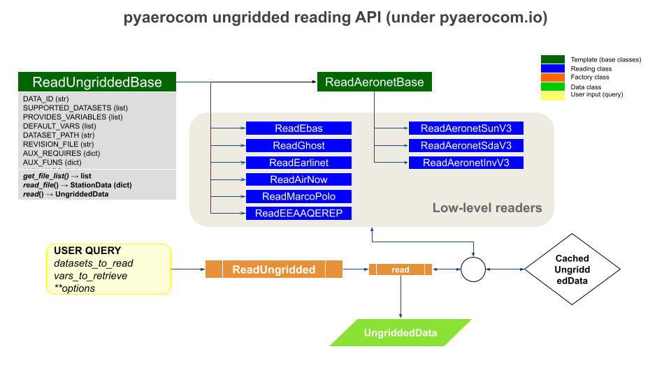
The actual classes handling the reading of data (for a given dataset) are indicated in blue. The orange ReadUngridded class is a factory class, that knows about the blue reading classes via a unique ID (similar to the gridded reading). Thus, as indicated, as a user, you do not need to know which exact reading class you need, you just need the ID and ReadUngridded will know which (blue) reader to use. To summarise, what you need for reading an ungridded dataset is:
- A path where the actual datafiles are located
- An unique ID, that links that path with a name
- A reader that can read the class
The first 2 points are available via:
pya.const.OBSLOCS_UNGRIDDED
OrderedDict([('AeronetSunV2Lev1.5.daily', '/lustre/storeA/project/aerocom/'),
             ('AeronetSun_2.0_NRT',
              '/lustre/storeA/project/aerocom/aerocom1/AEROCOM_OBSDATA/AeronetSunNRT'),
             ('AeronetSunV2Lev2.daily',
              '/lustre/storeA/project/aerocom/aerocom1/AEROCOM_OBSDATA/AeronetRaw2.0/renamed'),
             ('AeronetSunV2Lev2.AP',
              '/lustre/storeA/project/aerocom/aerocom1/AEROCOM_OBSDATA/AeronetSun2.0AllPoints/renamed'),
             ('AeronetSDAV2Lev2.daily',
              '/lustre/storeA/project/aerocom/aerocom1/AEROCOM_OBSDATA/AeronetSun2.0.SDA.daily/renamed'),
             ('AeronetSDAV2Lev2.AP',
              '/lustre/storeA/project/aerocom/aerocom1/AEROCOM_OBSDATA/AeronetSun2.0.SDA.AP/renamed'),
             ('AeronetInvV2Lev1.5.daily',
              '/lustre/storeA/project/aerocom/aerocom1/AEROCOM_OBSDATA/Aeronet.Inv.V2L1.5.daily/renamed'),
             ('AeronetInvV2Lev1.5.AP',
              '/lustre/storeA/project/aerocom/aerocom1/AEROCOM_OBSDATA/'),
             ('AeronetInvV2Lev2.daily',
              '/lustre/storeA/project/aerocom/aerocom1/AEROCOM_OBSDATA/Aeronet.Inv.V2L2.0.daily/renamed'),
             ('AeronetInvV2Lev2.AP',
              '/lustre/storeA/project/aerocom/aerocom1/AEROCOM_OBSDATA/'),
             ('AeronetSunV3Lev1.5.daily',
              '/lustre/storeA/project/aerocom/aerocom1/AEROCOM_OBSDATA/AeronetSunV3Lev1.5.daily/renamed'),
             ('AeronetSunV3Lev1.5.AP',
              '/lustre/storeA/project/aerocom/aerocom1/AEROCOM_OBSDATA/AeronetSunV3Lev1.5.AP/renamed'),
             ('AeronetSunV3Lev2.daily',
              '/lustre/storeA/project/aerocom/aerocom1/AEROCOM_OBSDATA/AeronetSunV3Lev2.0.daily/renamed'),
             ('AeronetSunV3Lev2.AP',
              '/lustre/storeA/project/aerocom/aerocom1/AEROCOM_OBSDATA/AeronetSunV3Lev2.0.AP/renamed'),
             ('AeronetSDAV3Lev1.5.daily',
              '/lustre/storeA/project/aerocom/aerocom1/AEROCOM_OBSDATA/Aeronet.SDA.V3L1.5.daily/renamed'),
             ('AeronetSDAV3Lev1.5.AP',
              '/lustre/storeA/project/aerocom/aerocom1/AEROCOM_OBSDATA/'),
             ('AeronetSDAV3Lev2.daily',
              '/lustre/storeA/project/aerocom/aerocom1/AEROCOM_OBSDATA/Aeronet.SDA.V3L2.0.daily/renamed'),
             ('AeronetSDAV3Lev2.AP',
              '/lustre/storeA/project/aerocom/aerocom1/AEROCOM_OBSDATA/'),
             ('AeronetInvV3Lev1.5.daily',
              '/lustre/storeA/project/aerocom/aerocom1/AEROCOM_OBSDATA/Aeronet.Inv.V3L1.5.daily/renamed'),
             ('AeronetInvV3Lev2.daily',
              '/lustre/storeA/project/aerocom/aerocom1/AEROCOM_OBSDATA/Aeronet.Inv.V3L2.0.daily/renamed'),
             ('EBASMC',
              '/lustre/storeA/project/aerocom/aerocom1/AEROCOM_OBSDATA/EBASMultiColumn/data'),
             ('EEAAQeRep',
              '/lustre/storeA/project/aerocom/aerocom1/AEROCOM_OBSDATA/EEA_AQeRep/renamed'),
             ('EARLINET',
              '/lustre/storeA/project/aerocom/aerocom1/AEROCOM_OBSDATA/Export/Earlinet/CAMS/data'),
             ('GAWTADsubsetAasEtAl',
              '/lustre/storeA/project/aerocom/aerocom1/AEROCOM_OBSDATA/PYAEROCOM/GAWTADSulphurSubset/data'),
             ('DMS_AMS_CVO',
              '/lustre/storeA/project/aerocom/aerocom1/AEROCOM_OBSDATA/PYAEROCOM/DMS_AMS_CVO/data'),
             ('GHOST.EEA.daily',
              '/lustre/storeA/project/aerocom/aerocom1/AEROCOM_OBSDATA/GHOST/data/EEA_AQ_eReporting/daily'),
             ('GHOST.EEA.hourly',
              '/lustre/storeA/project/aerocom/aerocom1/AEROCOM_OBSDATA/GHOST/data/EEA_AQ_eReporting/hourly'),
             ('GHOST.EEA.monthly',
              '/lustre/storeA/project/aerocom/aerocom1/AEROCOM_OBSDATA/GHOST/data/EEA_AQ_eReporting/monthly'),
             ('GHOST.EBAS.daily',
              '/lustre/storeA/project/aerocom/aerocom1/AEROCOM_OBSDATA/GHOST/data/EBAS/daily'),
             ('GHOST.EBAS.hourly',
              '/lustre/storeA/project/aerocom/aerocom1/AEROCOM_OBSDATA/GHOST/data/EBAS/hourly'),
             ('GHOST.EBAS.monthly',
              '/lustre/storeA/project/aerocom/aerocom1/AEROCOM_OBSDATA/GHOST/data/EBAS/monthly'),
             ('EEAAQeRep.NRT',
              '/lustre/storeA/project/aerocom/aerocom1/AEROCOM_OBSDATA/EEA_AQeRep.NRT/renamed/'),
             ('EEAAQeRep.v2',
              '/lustre/storeA/project/aerocom/aerocom1/AEROCOM_OBSDATA/EEA_AQeRep.v2/renamed/'),
             ('AirNow',
              '/lustre/storeA/project/aerocom/aerocom1/AEROCOM_OBSDATA/MACC_INSITU_AirNow'),
             ('MarcoPolo',
              '/lustre/storeA/project/aerocom/aerocom1/AEROCOM_OBSDATA/CHINA_MP_NRT'),
             ('AeronetSunV3L2Subset.daily',
              '/home/jonasg/MyPyaerocom/testdata-minimal/obsdata/AeronetSunV3Lev2.daily/renamed'),
             ('AeronetSDAV3L2Subset.daily',
              '/home/jonasg/MyPyaerocom/testdata-minimal/obsdata/AeronetSDAV3Lev2.daily/renamed'),
             ('AeronetInvV3L2Subset.daily',
              '/home/jonasg/MyPyaerocom/testdata-minimal/obsdata/AeronetInvV3Lev2.daily/renamed'),
             ('EBASSubset',
              '/home/jonasg/MyPyaerocom/testdata-minimal/obsdata/EBASMultiColumn'),
             ('AirNowSubset',
              '/home/jonasg/MyPyaerocom/testdata-minimal/obsdata/AirNowSubset'),
             ('G.EEA.daily.Subset',
              '/home/jonasg/MyPyaerocom/testdata-minimal/obsdata/GHOST/data/EEA_AQ_eReporting/daily'),
             ('G.EEA.hourly.Subset',
              '/home/jonasg/MyPyaerocom/testdata-minimal/obsdata/GHOST/data/EEA_AQ_eReporting/hourly'),
             ('G.EBAS.daily.Subset',
              '/home/jonasg/MyPyaerocom/testdata-minimal/obsdata/GHOST/data/EBAS/daily'),
             ('G.EBAS.hourly.Subset',
              '/home/jonasg/MyPyaerocom/testdata-minimal/obsdata/GHOST/data/EBAS/hourly')])
And the reader classes that are supposed to be used for each of these IDs is provided in the ReadUngridded class header:
pya.io.ReadUngridded.SUPPORTED_READERS
[pyaerocom.io.read_aeronet_invv3.ReadAeronetInvV3,
 pyaerocom.io.read_aeronet_invv2.ReadAeronetInvV2,
 pyaerocom.io.read_aeronet_sdav2.ReadAeronetSdaV2,
 pyaerocom.io.read_aeronet_sdav3.ReadAeronetSdaV3,
 pyaerocom.io.read_aeronet_sunv2.ReadAeronetSunV2,
 pyaerocom.io.read_aeronet_sunv3.ReadAeronetSunV3,
 pyaerocom.io.read_earlinet.ReadEarlinet,
 pyaerocom.io.read_ebas.ReadEbas,
 pyaerocom.io.read_gaw.ReadGAW,
 pyaerocom.io.read_aasetal.ReadAasEtal,
 pyaerocom.io.read_ghost.ReadGhost,
 pyaerocom.io.read_airnow.ReadAirNow,
 pyaerocom.io.read_marcopolo.ReadMarcoPolo,
 pyaerocom.io.read_eea_aqerep.ReadEEAAQEREP,
 pyaerocom.io.read_eea_aqerep_v2.ReadEEAAQEREP_V2]
The link between ID (keys of const.OBSLOCS_UNGRIDDED) and reader is available in the actual readers themselves, e.g.:
pya.io.read_aeronet_sunv3.ReadAeronetSunV3.SUPPORTED_DATASETS
['AeronetSunV3Lev1.5.daily',
 'AeronetSunV3Lev1.5.AP',
 'AeronetSunV3Lev2.daily',
 'AeronetSunV3Lev2.AP',
 'AeronetSunV3L2Subset.daily']
But these are details that you usually do not need to worry about. If you want to register a new observation dataset, you need the 3 points specified above and can add it via:
aeronet_sun_datadir = f'{pya.const.OUTPUTDIR}/testdata-minimal/obsdata/AeronetSunV3Lev2.daily/renamed'
pya.const.add_ungridded_obs(obs_id='Bla',
                            data_dir=aeronet_sun_datadir,
                            reader=pya.io.read_aeronet_sunv3.ReadAeronetSunV3)
Now, we basically have 2 names for the same dataset:
pya.io.read_aeronet_sunv3.ReadAeronetSunV3.SUPPORTED_DATASETS
['AeronetSunV3Lev1.5.daily',
 'AeronetSunV3Lev1.5.AP',
 'AeronetSunV3Lev2.daily',
 'AeronetSunV3Lev2.AP',
 'AeronetSunV3L2Subset.daily',
 'Bla']
That is, the data under the above directory is now accessible via 2 IDs: Bla and AeronetSunV3L2Subset.daily.
Before continuing with the reading of observational data, some things need to be said related to the caching of UngriddedData objects.
Caching of UngriddedData
Reading of ungridded data is often rather time-consuming. Therefore, pyaerocom uses a caching strategy that stores loaded instances of the UngriddedData class as pickle files in a cache directory (illustrated in the flowchart shown above). The loaction of the cache directory can be accessed via:
pya.const.CACHEDIR
'/home/jonasg/MyPyaerocom/_cache/jonasg'
You may change this directory if required.
f'Caching is active? {pya.const.CACHING}'
'Caching is active? True'
Deactivate / Activate caching
pya.const.CACHING = False
pya.const.CACHING = True
Note: if caching is active, make sure you have enough disk quota or change location where the cache files are stored.
Read Aeronet Sun v3 level 2 data
As illustrated in the flowchart above, ungridded observation data can be imported using the ReadUngridded class. Like for the model data, observation datasets can be searched as follows:
pya.browse_database('Aeronet*');
Found more than 20 matches for input pattern Aeronet*:

Matches: ['AeronetSunV2Lev1.5.daily', 'AeronetSun_2.0_NRT', 'AeronetSunV2Lev2.daily', 'AeronetSunV2Lev2.AP', 'AeronetSDAV2Lev2.daily', 'AeronetInvV2Lev1.5.daily', 'AeronetInvV2Lev1.5.AP', 'AeronetInvV2Lev2.daily', 'AeronetInvV2Lev2.AP', 'AeronetSunV3Lev1.5.daily', 'AeronetSunV3Lev1.5.AP', 'AeronetSunV3Lev2.daily', 'AeronetSunV3Lev2.AP', 'AeronetSDAV3Lev1.5.daily', 'AeronetSDAV3Lev1.5.AP', 'AeronetSDAV3Lev2.daily', 'AeronetSDAV3Lev2.AP', 'AeronetInvV3Lev1.5.daily', 'AeronetInvV3Lev2.daily', 'AeronetSunV3L2Subset.daily', 'AeronetSDAV3L2Subset.daily', 'AeronetInvV3L2Subset.daily', 'AERONET_TESTBED-SK']

To receive more detailed information, please specify search ID more accurately
The search routine found 3 matches for the 3 different AERONET data products: Sun, SDA, and Inv (inversion). You may read more about the different products at the AERONET website.
Let's continue with the "Sun" product (AERONET Direct Sun algorithm). As you can see from the output above, this dataset contains daily averages, which is convenient to use for model evaluation.
obs_id = 'AeronetSunV3L2Subset.daily'
obs_reader = pya.io.ReadUngridded(obs_id)
print(obs_reader)
Dataset name: AeronetSunV3L2Subset.daily
Data directory: /home/jonasg/MyPyaerocom/testdata-minimal/obsdata/AeronetSunV3Lev2.daily/renamed
Supported variables: ['od340aer', 'od440aer', 'od500aer', 'od870aer', 'ang4487aer', 'ang44&87aer', 'od550aer']
Last revision: n/d
Let's read the data (you can read a single or multiple variables at the same time). For now, we only read the AOD at 550 nm:
od550aer_aeronet = obs_reader.read(vars_to_retrieve='od550aer')
od550aer_aeronet
UngriddedData <networks: ['AeronetSunV3L2Subset.daily']; vars: ['od550aer']; instruments: ['sun_photometer'];No. of metadata units: 22
As you can see, the data object is of type UngriddedData. Other than GriddedData, UngriddedData can hold an arbitrary number of variables, and even networks. The number of metadata units indicates the number of data files that have been read.
Plot all station coordinates
To get an overview, you can plot all site coordinates contained in the dataset. You can also plot multiple times into the same map with different input criteria. For instance, below we first plot all site locations available in the data (in red), and then, on top of it, in green, we plot sites that contain data in 2010.
ax = od550aer_aeronet.plot_station_coordinates(markersize=80)
od550aer_aeronet.plot_station_coordinates(color='lime', var_name='od550aer', start=2010, stop=2011, markersize=20, ax=ax)
<GeoAxes:title={'center':'od550aer_01.01.2010-31.12.2010'}, xlabel='Longitude', ylabel='Latitude'>

Access of individual stations
For intercomparison with model data, we are interested in time-series from individual sites. You can check out all existing site-location names via:
od550aer_aeronet.unique_station_names
['AAOT',
 'ARIAKE_TOWER',
 'Agoufou',
 'Alta_Floresta',
 'American_Samoa',
 'Amsterdam_Island',
 'Anmyon',
 'Avignon',
 'Azores',
 'BORDEAUX',
 'Barbados',
 'Blyth_NOAH',
 'La_Paz',
 'Mauna_Loa',
 'Tahiti',
 'Taihu',
 'Taipei_CWB',
 'Tamanrasset_INM',
 'The_Hague',
 'Thessaloniki',
 'Thornton_C-power',
 'Trelew']
To access individual site location data as StationData you can simply do:
station_data = od550aer_aeronet['La_Paz'] # this is fully equivalent with aeronet_data.to_station_data('Leipzig')
station_data
StationData: {'dtime': array(['2006-02-18T00:00:00.000000000', '2006-02-19T00:00:00.000000000',
       '2006-02-20T00:00:00.000000000', ...,
       '2019-05-24T00:00:00.000000000', '2019-05-25T00:00:00.000000000',
       '2019-05-26T00:00:00.000000000'], dtype='datetime64[ns]'), 'var_info': BrowseDict: {'od550aer': OrderedDict([('units', '1'), ('overlap', False), ('ts_type', 'daily'), ('min_num_obs', None), ('how', 'mean')])}, 'station_coords': {'latitude': -16.538999999999998, 'longitude': -68.066467, 'altitude': 3439.0}, 'data_err': BrowseDict: {}, 'overlap': BrowseDict: {}, 'numobs': BrowseDict: {}, 'data_flagged': BrowseDict: {}, 'filename': '/home/jonasg/MyPyaerocom/testdata-minimal/obsdata/AeronetSunV3Lev2.daily/renamed/La_Paz.lev30', 'station_id': None, 'station_name': 'La_Paz', 'instrument_name': 'sun_photometer', 'PI': 'Brent_Holben', 'country': None, 'country_code': None, 'ts_type': 'daily', 'latitude': -16.538999999999998, 'longitude': -68.066467, 'altitude': 3439.0, 'data_id': 'AeronetSunV3L2Subset.daily', 'dataset_name': None, 'data_product': None, 'data_version': None, 'data_level': None, 'framework': None, 'instr_vert_loc': None, 'revision_date': None, 'website': None, 'ts_type_src': 'daily', 'stat_merge_pref_attr': None, 'data_revision': 'n/d', 'od550aer': 2006-02-18    0.087568
2006-02-19         NaN
2006-02-20         NaN
2006-02-21         NaN
2006-02-22    0.101807
                ...
2019-05-22         NaN
2019-05-23    0.059489
2019-05-24    0.049292
2019-05-25    0.074172
2019-05-26    0.060137
Freq: D, Length: 4846, dtype: float64}
As you can see, the returned object is of type StationData which has been introduced above (remember, we extracted a time series from the TM5 model for the location of Oslo).
As mentioned above, it can be used like a dictionary, and the variable time-series can be accessed via:
station_data['od550aer'].plot()
<AxesSubplot:>

You may also plot directly from the StationData object (and do some more other hopefully self-explanatory things):
ax = station_data.plot_timeseries('od550aer', marker='x', ls='none')
station_data.resample_time(var_name='od550aer', ts_type='monthly').plot_timeseries('od550aer', marker=' ', ls='-', lw=3, ax=ax)
<AxesSubplot:title={'center':'La_Paz'}, ylabel='od550aer'>

Back to UngriddedData: You may also retrieve the StationData with specifying more constraints using to_station_data (e.g. in monthly resolution and only for the year 2010). And you can overlay different curves, by passing the axes instance returned by the plotting method:
ax=od550aer_aeronet.to_station_data('La_Paz',
                                    start=2010, stop=2011,
                                    freq='daily').plot_timeseries('od550aer')

ax=od550aer_aeronet.to_station_data('La_Paz',
                                    start=2010,
                                    freq='monthly').plot_timeseries('od550aer', ax=ax)
ax.legend()
ax.set_title('La Paz AODs 2010');

You can also plot the time-series directly from UngriddedData
od550aer_aeronet.plot_station_timeseries('La_Paz', 'od550aer', ts_type='monthly',
                                     start=2018).set_title('Monthly AOD in La Paz, 2018');

Computing trends (BETA API, will likely see some revisions)
Trends can be computed using the same methodolgy as Mortier et al., 2020, which is also used in the Aerosol trends interface. You may also read about the method in the methods section therein.
te = pya.trends_engine.TrendsEngine
timeseries_monthly = station_data.resample_time('od550aer', ts_type='monthly')['od550aer']
result = te.compute_trend(data=timeseries_monthly, start_year=2008, stop_year=2019, ts_type='monthly', min_num_yrs=7)
result
{'pval': 0.12097096961680295,
 'm': -0.0017985318700550548,
 'm_err': 0.0016087563002642336,
 'n': 11,
 'y_mean': 0.09864413175599861,
 'y_min': 0.07926316386912101,
 'y_max': 0.1684956149220456,
 'slp': -1.782064278905696,
 'slp_err': 1.6112865430184924,
 'reg0': 0.10092407391496962,
 'slp_2008': -1.782064278905696,
 'slp_2008_err': 1.6112865430184924,
 'reg0_2008': 0.10092407391496962,
 'data': 2008-06-15    0.091931
 2009-06-15    0.168496
 2010-06-15    0.113513
 2011-06-15    0.099361
 2012-06-15    0.086237
 2013-06-15    0.079263
 2014-06-15    0.094324
 2015-06-15    0.081144
 2016-06-15    0.090727
 2017-06-15    0.093958
 2018-06-15    0.086130
 2019-06-15         NaN
 dtype: float64,
 'period': '2008-2019',
 'season': 'all',
 'yoffs': 0.1692682849770617}
Colocation of model and obsdata
Now that we have a gridded model dataset and an ungridded observation dataset loaded we can continue with colocation of both datasets. Colocation essentially describes the process of matching observations and model in space and time, which makes it possible to compare both and ultimately, to assess how well the model is performing.
As the observations are usually sparse, they define the set of locations and times to be extracted from the model (for comparison). Essentially, what needs to be done is simple:
- Decide on a time interval in which you want to colocate the observations with the model data.
- Decide on an output frequency.
- Find all site location coordinates from the observations in the time period and extract the model values from the model dataset at these locations.
- Match the time interval and frequency.
pyaerocom has some methods that can do this for you and these methods return an instance of the ColocatedData object.
Low-level colocation routine(s)
Let's colocate the TM5 model data with the AERONET AOD subset for the year 2010 and in monthly resolution. Since we already have both data objects loaded, we can go straight to the low-level colocation routine:
coldata = pya.colocation.colocate_gridded_ungridded(od550aer_tm5,
                                                    od550aer_aeronet,
                                                    ts_type='monthly',
                                                    start=2010,
                                                    filter_name='WORLD-noMOUNTAINS')
/home/jonasg/github/pya/pyaerocom/pyaerocom/ungriddeddata.py:137: RuntimeWarning: invalid value encountered in multiply
  self._data = np.empty([num_points, self._COLNO]) * np.nan
The filter-name WORLD-noMOUNTAINS denotes that all available AERONET sites are supposed to be used but high altitude sites (located above 1000m a.s.l). A more detailed introduction into available regions and region filters is provided in the getting_started_setup.ipynb tutorial.
You may create a scatter plot from these colocated monthly means, which includes relevant statistical parameters that help to assess model performance:
coldata.plot_scatter(loglog=True);

Does not look too bad, you can see that this result is from 8 sites and 62 data points (monthly averages). The normalised-mean-bias (NMB) is -15.5%, which means that the model slightly underestimates AOD at these locations.
A more illustrative view of the model biases can be retrieved by plotting a bias map:
pya.plot.mapping.plot_nmb_map_colocateddata(coldata);

The fact that you can barely see most of the sites is a good sign, since 0% bias is mapped to white color which is the same as the background color here. The largest bias is found in Amsterdam Island, in the southern Indian Ocean, which could be an indication that the model is simulating too little sea-salt aerosol in this very remote and clean region.
Under the hood ...
... the ColocatedData object is an xarray.DataArray:
coldata.data
<xarray.DataArray 'od550aer' (data_source: 2, time: 12, station_name: 8)>
array([[[       nan, 0.10766512, 0.03649583, 0.11300932,        nan,
                nan, 0.13828996, 0.03593528],
        [       nan, 0.1281071 , 0.05131321, 0.1490295 , 0.58044357,
         0.88151395, 0.09390731, 0.03669082],
        [       nan, 0.06650846, 0.05941147, 0.15400053, 0.77145611,
         0.81960458, 0.15375983, 0.03303893],
        [1.04184348, 0.09195735, 0.17511331, 0.17945707, 0.56584754,
         0.66320834, 0.26381093, 0.03862473],
        [1.05366664, 0.0922461 , 0.18108093, 0.13238964, 0.62159417,
         0.49044907, 0.18389999,        nan],
        [1.00704245,        nan, 0.23711979, 0.12935421, 1.01970277,
         0.43910105, 0.23285789,        nan],
        [0.98468077,        nan, 0.28315152, 0.15569135, 0.57586237,
                nan, 0.22223999,        nan],
        [0.34698175, 1.1291196 , 0.22721504, 0.1078829 , 0.6659021 ,
                nan, 0.28657127, 0.03157442],
        [0.34638257, 1.36759564, 0.22911738, 0.12730093, 0.48163878,
                nan, 0.17283706, 0.05573316],
        [       nan, 0.51974499, 0.19571329, 0.19495548,        nan,
                nan, 0.14301278, 0.06043777],
...
        [0.89635843, 0.07341532, 0.06992208, 0.14702028, 1.00326443,
         0.63314253, 0.22872289, 0.05543199],
        [0.77087325, 0.1048945 , 0.06650965, 0.1865073 , 0.7776224 ,
         0.54631037, 0.28632328, 0.03336016],
        [0.80734402, 0.12378095, 0.05653326, 0.17420147, 0.65254241,
         0.45009974, 0.30526772, 0.03229909],
        [0.50654256, 0.14234523, 0.06274261, 0.17343882, 0.58004749,
         0.33348686, 0.30070606, 0.03174512],
        [0.46850282, 0.1863786 , 0.0675569 , 0.17624108, 0.47164536,
         0.19874078, 0.24717812, 0.04090422],
        [0.34062195, 1.90581691, 0.07018556, 0.15123938, 0.36946237,
         0.18504179, 0.26474383, 0.03088068],
        [0.24573354, 1.21507001, 0.11556577, 0.13191637, 0.4020009 ,
         0.26275966, 0.23841298, 0.04008143],
        [0.2798166 , 0.15733013, 0.08971586, 0.13991331, 0.38702768,
         0.34291422, 0.21531013, 0.03859388],
        [0.35316458, 0.08011972, 0.0626139 , 0.069165  , 0.55920124,
         0.38426778, 0.19802441, 0.03579372],
        [0.28721237, 0.0827378 , 0.07033022, 0.07274448, 0.50464362,
         0.3815313 , 0.1641538 , 0.04502364]]])
Coordinates:
  * data_source   (data_source) <U26 'AeronetSunV3L2Subset.daily' 'TM5-met201...
  * time          (time) datetime64[ns] 2010-01-15 2010-02-15 ... 2010-12-15
  * station_name  (station_name) <U16 'Agoufou' 'Alta_Floresta' ... 'Trelew'
    latitude      (station_name) float64 15.35 -9.871 -37.8 ... 40.63 -43.25
    longitude     (station_name) float64 -1.479 -56.1 77.57 ... 22.96 -65.31
    altitude      (station_name) float64 305.0 277.0 49.0 ... 26.0 60.0 15.0
Attributes: (12/16)
    data_source:     ['AeronetSunV3L2Subset.daily', 'TM5-met2010_CTRL-TEST']
    var_name:        ['od550aer', 'od550aer']
    var_name_input:  ['od550aer', 'od550aer']
    ts_type:         monthly
    filter_name:     WORLD-noMOUNTAINS
    ts_type_src:     ['daily', 'monthly']
    ...              ...
    from_files_ref:  None
    colocate_time:   False
    obs_is_clim:     False
    pyaerocom:       0.12.0.dev1
    min_num_obs:     None
resample_how: None- data_source: 2
- time: 12
- station_name: 8
- nan 0.1077 0.0365 0.113 nan ... 0.07274 0.5046 0.3815 0.1642 0.04502
array([[[ nan, 0.10766512, 0.03649583, 0.11300932, nan, nan, 0.13828996, 0.03593528], [ nan, 0.1281071 , 0.05131321, 0.1490295 , 0.58044357, 0.88151395, 0.09390731, 0.03669082], [ nan, 0.06650846, 0.05941147, 0.15400053, 0.77145611, 0.81960458, 0.15375983, 0.03303893], [1.04184348, 0.09195735, 0.17511331, 0.17945707, 0.56584754, 0.66320834, 0.26381093, 0.03862473], [1.05366664, 0.0922461 , 0.18108093, 0.13238964, 0.62159417, 0.49044907, 0.18389999, nan], [1.00704245, nan, 0.23711979, 0.12935421, 1.01970277, 0.43910105, 0.23285789, nan], [0.98468077, nan, 0.28315152, 0.15569135, 0.57586237, nan, 0.22223999, nan], [0.34698175, 1.1291196 , 0.22721504, 0.1078829 , 0.6659021 , nan, 0.28657127, 0.03157442], [0.34638257, 1.36759564, 0.22911738, 0.12730093, 0.48163878, nan, 0.17283706, 0.05573316], [ nan, 0.51974499, 0.19571329, 0.19495548, nan, nan, 0.14301278, 0.06043777], ... [0.89635843, 0.07341532, 0.06992208, 0.14702028, 1.00326443, 0.63314253, 0.22872289, 0.05543199], [0.77087325, 0.1048945 , 0.06650965, 0.1865073 , 0.7776224 , 0.54631037, 0.28632328, 0.03336016], [0.80734402, 0.12378095, 0.05653326, 0.17420147, 0.65254241, 0.45009974, 0.30526772, 0.03229909], [0.50654256, 0.14234523, 0.06274261, 0.17343882, 0.58004749, 0.33348686, 0.30070606, 0.03174512], [0.46850282, 0.1863786 , 0.0675569 , 0.17624108, 0.47164536, 0.19874078, 0.24717812, 0.04090422], [0.34062195, 1.90581691, 0.07018556, 0.15123938, 0.36946237, 0.18504179, 0.26474383, 0.03088068], [0.24573354, 1.21507001, 0.11556577, 0.13191637, 0.4020009 , 0.26275966, 0.23841298, 0.04008143], [0.2798166 , 0.15733013, 0.08971586, 0.13991331, 0.38702768, 0.34291422, 0.21531013, 0.03859388], [0.35316458, 0.08011972, 0.0626139 , 0.069165 , 0.55920124, 0.38426778, 0.19802441, 0.03579372], [0.28721237, 0.0827378 , 0.07033022, 0.07274448, 0.50464362, 0.3815313 , 0.1641538 , 0.04502364]]]) - data_source(data_source)<U26'AeronetSunV3L2Subset.daily' 'TM...
array(['AeronetSunV3L2Subset.daily', 'TM5-met2010_CTRL-TEST'], dtype='<U26')
- time(time)datetime64[ns]2010-01-15 ... 2010-12-15
array(['2010-01-15T00:00:00.000000000', '2010-02-15T00:00:00.000000000', '2010-03-15T00:00:00.000000000', '2010-04-15T00:00:00.000000000', '2010-05-15T00:00:00.000000000', '2010-06-15T00:00:00.000000000', '2010-07-15T00:00:00.000000000', '2010-08-15T00:00:00.000000000', '2010-09-15T00:00:00.000000000', '2010-10-15T00:00:00.000000000', '2010-11-15T00:00:00.000000000', '2010-12-15T00:00:00.000000000'], dtype='datetime64[ns]') - station_name(station_name)<U16'Agoufou' ... 'Trelew'
array(['Agoufou', 'Alta_Floresta', 'Amsterdam_Island', 'Avignon', 'Taihu', 'Taipei_CWB', 'Thessaloniki', 'Trelew'], dtype='<U16') - latitude(station_name)float6415.35 -9.871 -37.8 ... 40.63 -43.25
- standard_name :
- latitude
- units :
- degrees
array([ 15.3454 , -9.871339, -37.799544, 43.93275 , 31.421 , 25.014683, 40.63 , -43.249806]) - longitude(station_name)float64-1.479 -56.1 77.57 ... 22.96 -65.31
- standard_name :
- longitude
- units :
- degrees
array([ -1.479117, -56.104453, 77.571946, 4.878067, 120.215333, 121.53837 , 22.96 , -65.308611]) - altitude(station_name)float64305.0 277.0 49.0 ... 26.0 60.0 15.0
array([305., 277., 49., 32., 20., 26., 60., 15.])
- data_source :
- ['AeronetSunV3L2Subset.daily', 'TM5-met2010_CTRL-TEST']
- var_name :
- ['od550aer', 'od550aer']
- var_name_input :
- ['od550aer', 'od550aer']
- ts_type :
- monthly
- filter_name :
- WORLD-noMOUNTAINS
- ts_type_src :
- ['daily', 'monthly']
- var_units :
- ['1', '1']
- data_level :
- 3
- revision_ref :
- n/d
- from_files :
- ['aerocom3_TM5_AP3-CTRL2016_od550aer_Column_2010_monthly.nc']
- from_files_ref :
- None
- colocate_time :
- False
- obs_is_clim :
- False
- pyaerocom :
- 0.12.0.dev1
- min_num_obs :
- None
- resample_how :
- None
As you can see, model and obs (stored in data_source dimension) now share the same coordinates (dimension station_name) and time stamps (dimension time). The data_source dimension always contains the observation data at the first index and the model data at the second:
obsdata = coldata.data[0]
obsdata
<xarray.DataArray 'od550aer' (time: 12, station_name: 8)>
array([[       nan, 0.10766512, 0.03649583, 0.11300932,        nan,
               nan, 0.13828996, 0.03593528],
       [       nan, 0.1281071 , 0.05131321, 0.1490295 , 0.58044357,
        0.88151395, 0.09390731, 0.03669082],
       [       nan, 0.06650846, 0.05941147, 0.15400053, 0.77145611,
        0.81960458, 0.15375983, 0.03303893],
       [1.04184348, 0.09195735, 0.17511331, 0.17945707, 0.56584754,
        0.66320834, 0.26381093, 0.03862473],
       [1.05366664, 0.0922461 , 0.18108093, 0.13238964, 0.62159417,
        0.49044907, 0.18389999,        nan],
       [1.00704245,        nan, 0.23711979, 0.12935421, 1.01970277,
        0.43910105, 0.23285789,        nan],
       [0.98468077,        nan, 0.28315152, 0.15569135, 0.57586237,
               nan, 0.22223999,        nan],
       [0.34698175, 1.1291196 , 0.22721504, 0.1078829 , 0.6659021 ,
               nan, 0.28657127, 0.03157442],
       [0.34638257, 1.36759564, 0.22911738, 0.12730093, 0.48163878,
               nan, 0.17283706, 0.05573316],
       [       nan, 0.51974499, 0.19571329, 0.19495548,        nan,
               nan, 0.14301278, 0.06043777],
       [       nan, 0.20634955, 0.18329662, 0.09995729,        nan,
               nan, 0.18381835, 0.04511684],
       [       nan, 0.17557466, 0.04773335, 0.10730821,        nan,
               nan, 0.19721314, 0.04412376]])
Coordinates:
    data_source   <U26 'AeronetSunV3L2Subset.daily'
  * time          (time) datetime64[ns] 2010-01-15 2010-02-15 ... 2010-12-15
  * station_name  (station_name) <U16 'Agoufou' 'Alta_Floresta' ... 'Trelew'
    latitude      (station_name) float64 15.35 -9.871 -37.8 ... 40.63 -43.25
    longitude     (station_name) float64 -1.479 -56.1 77.57 ... 22.96 -65.31
    altitude      (station_name) float64 305.0 277.0 49.0 ... 26.0 60.0 15.0
Attributes: (12/16)
    data_source:     ['AeronetSunV3L2Subset.daily', 'TM5-met2010_CTRL-TEST']
    var_name:        ['od550aer', 'od550aer']
    var_name_input:  ['od550aer', 'od550aer']
    ts_type:         monthly
    filter_name:     WORLD-noMOUNTAINS
    ts_type_src:     ['daily', 'monthly']
    ...              ...
    from_files_ref:  None
    colocate_time:   False
    obs_is_clim:     False
    pyaerocom:       0.12.0.dev1
    min_num_obs:     None
resample_how: None- time: 12
- station_name: 8
- nan 0.1077 0.0365 0.113 nan nan ... 0.1073 nan nan 0.1972 0.04412
array([[ nan, 0.10766512, 0.03649583, 0.11300932, nan, nan, 0.13828996, 0.03593528], [ nan, 0.1281071 , 0.05131321, 0.1490295 , 0.58044357, 0.88151395, 0.09390731, 0.03669082], [ nan, 0.06650846, 0.05941147, 0.15400053, 0.77145611, 0.81960458, 0.15375983, 0.03303893], [1.04184348, 0.09195735, 0.17511331, 0.17945707, 0.56584754, 0.66320834, 0.26381093, 0.03862473], [1.05366664, 0.0922461 , 0.18108093, 0.13238964, 0.62159417, 0.49044907, 0.18389999, nan], [1.00704245, nan, 0.23711979, 0.12935421, 1.01970277, 0.43910105, 0.23285789, nan], [0.98468077, nan, 0.28315152, 0.15569135, 0.57586237, nan, 0.22223999, nan], [0.34698175, 1.1291196 , 0.22721504, 0.1078829 , 0.6659021 , nan, 0.28657127, 0.03157442], [0.34638257, 1.36759564, 0.22911738, 0.12730093, 0.48163878, nan, 0.17283706, 0.05573316], [ nan, 0.51974499, 0.19571329, 0.19495548, nan, nan, 0.14301278, 0.06043777], [ nan, 0.20634955, 0.18329662, 0.09995729, nan, nan, 0.18381835, 0.04511684], [ nan, 0.17557466, 0.04773335, 0.10730821, nan, nan, 0.19721314, 0.04412376]]) - data_source()<U26'AeronetSunV3L2Subset.daily'
array('AeronetSunV3L2Subset.daily', dtype='<U26') - time(time)datetime64[ns]2010-01-15 ... 2010-12-15
array(['2010-01-15T00:00:00.000000000', '2010-02-15T00:00:00.000000000', '2010-03-15T00:00:00.000000000', '2010-04-15T00:00:00.000000000', '2010-05-15T00:00:00.000000000', '2010-06-15T00:00:00.000000000', '2010-07-15T00:00:00.000000000', '2010-08-15T00:00:00.000000000', '2010-09-15T00:00:00.000000000', '2010-10-15T00:00:00.000000000', '2010-11-15T00:00:00.000000000', '2010-12-15T00:00:00.000000000'], dtype='datetime64[ns]') - station_name(station_name)<U16'Agoufou' ... 'Trelew'
array(['Agoufou', 'Alta_Floresta', 'Amsterdam_Island', 'Avignon', 'Taihu', 'Taipei_CWB', 'Thessaloniki', 'Trelew'], dtype='<U16') - latitude(station_name)float6415.35 -9.871 -37.8 ... 40.63 -43.25
- standard_name :
- latitude
- units :
- degrees
array([ 15.3454 , -9.871339, -37.799544, 43.93275 , 31.421 , 25.014683, 40.63 , -43.249806]) - longitude(station_name)float64-1.479 -56.1 77.57 ... 22.96 -65.31
- standard_name :
- longitude
- units :
- degrees
array([ -1.479117, -56.104453, 77.571946, 4.878067, 120.215333, 121.53837 , 22.96 , -65.308611]) - altitude(station_name)float64305.0 277.0 49.0 ... 26.0 60.0 15.0
array([305., 277., 49., 32., 20., 26., 60., 15.])
- data_source :
- ['AeronetSunV3L2Subset.daily', 'TM5-met2010_CTRL-TEST']
- var_name :
- ['od550aer', 'od550aer']
- var_name_input :
- ['od550aer', 'od550aer']
- ts_type :
- monthly
- filter_name :
- WORLD-noMOUNTAINS
- ts_type_src :
- ['daily', 'monthly']
- var_units :
- ['1', '1']
- data_level :
- 3
- revision_ref :
- n/d
- from_files :
- ['aerocom3_TM5_AP3-CTRL2016_od550aer_Column_2010_monthly.nc']
- from_files_ref :
- None
- colocate_time :
- False
- obs_is_clim :
- False
- pyaerocom :
- 0.12.0.dev1
- min_num_obs :
- None
- resample_how :
- None
modeldata = coldata.data[1]
modeldata
<xarray.DataArray 'od550aer' (time: 12, station_name: 8)>
array([[0.15579131, 0.074198  , 0.07480989, 0.09742171, 0.51915187,
        0.32987517, 0.15443519, 0.04990007],
       [0.18340141, 0.0763083 , 0.07439816, 0.10789451, 0.49576023,
        0.36209598, 0.21525712, 0.05284398],
       [0.89635843, 0.07341532, 0.06992208, 0.14702028, 1.00326443,
        0.63314253, 0.22872289, 0.05543199],
       [0.77087325, 0.1048945 , 0.06650965, 0.1865073 , 0.7776224 ,
        0.54631037, 0.28632328, 0.03336016],
       [0.80734402, 0.12378095, 0.05653326, 0.17420147, 0.65254241,
        0.45009974, 0.30526772, 0.03229909],
       [0.50654256, 0.14234523, 0.06274261, 0.17343882, 0.58004749,
        0.33348686, 0.30070606, 0.03174512],
       [0.46850282, 0.1863786 , 0.0675569 , 0.17624108, 0.47164536,
        0.19874078, 0.24717812, 0.04090422],
       [0.34062195, 1.90581691, 0.07018556, 0.15123938, 0.36946237,
        0.18504179, 0.26474383, 0.03088068],
       [0.24573354, 1.21507001, 0.11556577, 0.13191637, 0.4020009 ,
        0.26275966, 0.23841298, 0.04008143],
       [0.2798166 , 0.15733013, 0.08971586, 0.13991331, 0.38702768,
        0.34291422, 0.21531013, 0.03859388],
       [0.35316458, 0.08011972, 0.0626139 , 0.069165  , 0.55920124,
        0.38426778, 0.19802441, 0.03579372],
       [0.28721237, 0.0827378 , 0.07033022, 0.07274448, 0.50464362,
        0.3815313 , 0.1641538 , 0.04502364]])
Coordinates:
    data_source   <U26 'TM5-met2010_CTRL-TEST'
  * time          (time) datetime64[ns] 2010-01-15 2010-02-15 ... 2010-12-15
  * station_name  (station_name) <U16 'Agoufou' 'Alta_Floresta' ... 'Trelew'
    latitude      (station_name) float64 15.35 -9.871 -37.8 ... 40.63 -43.25
    longitude     (station_name) float64 -1.479 -56.1 77.57 ... 22.96 -65.31
    altitude      (station_name) float64 305.0 277.0 49.0 ... 26.0 60.0 15.0
Attributes: (12/16)
    data_source:     ['AeronetSunV3L2Subset.daily', 'TM5-met2010_CTRL-TEST']
    var_name:        ['od550aer', 'od550aer']
    var_name_input:  ['od550aer', 'od550aer']
    ts_type:         monthly
    filter_name:     WORLD-noMOUNTAINS
    ts_type_src:     ['daily', 'monthly']
    ...              ...
    from_files_ref:  None
    colocate_time:   False
    obs_is_clim:     False
    pyaerocom:       0.12.0.dev1
    min_num_obs:     None
resample_how: None- time: 12
- station_name: 8
- 0.1558 0.0742 0.07481 0.09742 0.5192 ... 0.5046 0.3815 0.1642 0.04502
array([[0.15579131, 0.074198 , 0.07480989, 0.09742171, 0.51915187, 0.32987517, 0.15443519, 0.04990007], [0.18340141, 0.0763083 , 0.07439816, 0.10789451, 0.49576023, 0.36209598, 0.21525712, 0.05284398], [0.89635843, 0.07341532, 0.06992208, 0.14702028, 1.00326443, 0.63314253, 0.22872289, 0.05543199], [0.77087325, 0.1048945 , 0.06650965, 0.1865073 , 0.7776224 , 0.54631037, 0.28632328, 0.03336016], [0.80734402, 0.12378095, 0.05653326, 0.17420147, 0.65254241, 0.45009974, 0.30526772, 0.03229909], [0.50654256, 0.14234523, 0.06274261, 0.17343882, 0.58004749, 0.33348686, 0.30070606, 0.03174512], [0.46850282, 0.1863786 , 0.0675569 , 0.17624108, 0.47164536, 0.19874078, 0.24717812, 0.04090422], [0.34062195, 1.90581691, 0.07018556, 0.15123938, 0.36946237, 0.18504179, 0.26474383, 0.03088068], [0.24573354, 1.21507001, 0.11556577, 0.13191637, 0.4020009 , 0.26275966, 0.23841298, 0.04008143], [0.2798166 , 0.15733013, 0.08971586, 0.13991331, 0.38702768, 0.34291422, 0.21531013, 0.03859388], [0.35316458, 0.08011972, 0.0626139 , 0.069165 , 0.55920124, 0.38426778, 0.19802441, 0.03579372], [0.28721237, 0.0827378 , 0.07033022, 0.07274448, 0.50464362, 0.3815313 , 0.1641538 , 0.04502364]]) - data_source()<U26'TM5-met2010_CTRL-TEST'
array('TM5-met2010_CTRL-TEST', dtype='<U26') - time(time)datetime64[ns]2010-01-15 ... 2010-12-15
array(['2010-01-15T00:00:00.000000000', '2010-02-15T00:00:00.000000000', '2010-03-15T00:00:00.000000000', '2010-04-15T00:00:00.000000000', '2010-05-15T00:00:00.000000000', '2010-06-15T00:00:00.000000000', '2010-07-15T00:00:00.000000000', '2010-08-15T00:00:00.000000000', '2010-09-15T00:00:00.000000000', '2010-10-15T00:00:00.000000000', '2010-11-15T00:00:00.000000000', '2010-12-15T00:00:00.000000000'], dtype='datetime64[ns]') - station_name(station_name)<U16'Agoufou' ... 'Trelew'
array(['Agoufou', 'Alta_Floresta', 'Amsterdam_Island', 'Avignon', 'Taihu', 'Taipei_CWB', 'Thessaloniki', 'Trelew'], dtype='<U16') - latitude(station_name)float6415.35 -9.871 -37.8 ... 40.63 -43.25
- standard_name :
- latitude
- units :
- degrees
array([ 15.3454 , -9.871339, -37.799544, 43.93275 , 31.421 , 25.014683, 40.63 , -43.249806]) - longitude(station_name)float64-1.479 -56.1 77.57 ... 22.96 -65.31
- standard_name :
- longitude
- units :
- degrees
array([ -1.479117, -56.104453, 77.571946, 4.878067, 120.215333, 121.53837 , 22.96 , -65.308611]) - altitude(station_name)float64305.0 277.0 49.0 ... 26.0 60.0 15.0
array([305., 277., 49., 32., 20., 26., 60., 15.])
- data_source :
- ['AeronetSunV3L2Subset.daily', 'TM5-met2010_CTRL-TEST']
- var_name :
- ['od550aer', 'od550aer']
- var_name_input :
- ['od550aer', 'od550aer']
- ts_type :
- monthly
- filter_name :
- WORLD-noMOUNTAINS
- ts_type_src :
- ['daily', 'monthly']
- var_units :
- ['1', '1']
- data_level :
- 3
- revision_ref :
- n/d
- from_files :
- ['aerocom3_TM5_AP3-CTRL2016_od550aer_Column_2010_monthly.nc']
- from_files_ref :
- None
- colocate_time :
- False
- obs_is_clim :
- False
- pyaerocom :
- 0.12.0.dev1
- min_num_obs :
- None
- resample_how :
- None
High-level colocation routine
If it wasn't for the purpose of this notebook, normally, we don't want to go through the hassle of reading the data individually before colocating. Thus, pyaerocom has a high-level interface that can do colocation straight with the observation and model IDs (under the hood, of course, it uses the same routines that have been used here). By default, this high-level interface also stores all produced ColocatedData objects as NetCDF files, for later analysis:
colocator = pya.Colocator(
    model_id=model_id, obs_id=obs_id, obs_vars='od550aer',
    ts_type='monthly',
    model_ts_type_read='monthly',
    filter_name='OCN', #  let's try to better isolate Amsterdam Island
    reanalyse_existing=True,
    save_coldata=True)

colocator
Colocator: {'model_id': 'TM5-met2010_CTRL-TEST', 'obs_id': 'AeronetSunV3L2Subset.daily', 'obs_vars': ['od550aer'], 'ts_type': 'monthly', 'start': None, 'stop': None, 'filter_name': 'OCN', 'basedir_coldata': '/home/jonasg/MyPyaerocom/colocated_data', 'save_coldata': True, 'obs_name': None, 'obs_data_dir': None, 'obs_use_climatology': False, '_obs_cache_only': False, 'obs_vert_type': None, 'obs_ts_type_read': None, 'obs_filters': {}, 'read_opts_ungridded': {}, 'model_name': None, 'model_data_dir': None, 'model_vert_type_alt': None, 'model_read_opts': {}, 'model_use_vars': {}, 'model_rename_vars': {}, 'model_add_vars': {}, 'model_to_stp': False, 'model_ts_type_read': 'monthly', 'model_read_aux': {}, 'model_use_climatology': False, 'gridded_reader_id': {'model': 'ReadGridded', 'obs': 'ReadGridded'}, 'flex_ts_type': True, 'min_num_obs': None, 'resample_how': 'mean', 'obs_remove_outliers': False, 'model_remove_outliers': False, 'obs_outlier_ranges': {}, 'model_outlier_ranges': {}, 'zeros_to_nan': False, 'harmonise_units': False, 'regrid_res_deg': None, 'colocate_time': False, 'reanalyse_existing': True, 'raise_exceptions': False, 'keep_data': True, 'add_meta': {}, '_log': None, 'logging': True, '_loaded_model_data': {}, 'data': {}, '_processing_status': [], 'files_written': [], '_model_reader': None, '_obs_reader': None}
Quite a few options, a lot of them are for the even higher-level automatic web-processing tools that feed the Aerocom Evaluation websites, so let's not get lost in these details here.
The colocation can be run as follows:
colocator.run()
Rearranging longitude dimension from 0 -> 360 definition to -180 -> 180 definition
WARNING: Found definition of outlier ranges for od550aer (TM5-met2010_CTRL-TEST) but outlier removal is deactivated. Consider checking your setup (note: model or obs outlier removal can be activated via attrs. model_remove_outliers and remove_outliers, respectively
The following variable combinations will be colocated
MODEL-VAR	OBS-VAR
od550aer	od550aer
Running TM5-met2010_CTRL-TEST (od550aer) vs. AeronetSunV3L2Subset.daily (od550aer)
WRITE: /home/jonasg/MyPyaerocom/colocated_data/TM5-met2010_CTRL-TEST/od550aer_od550aer_MOD-TM5-met2010_CTRL-TEST_REF-AeronetSunV3L2Subset.daily_20100101_20101231_monthly_OCN.nc

Colocation processing status for TM5-met2010_CTRL-TEST vs. AeronetSunV3L2Subset.daily
  Model Var   Obs Var   Status
0  od550aer  od550aer  SUCCESS
{'od550aer': {'od550aer': pyaerocom.ColocatedData: data: <xarray.DataArray 'od550aer' (data_source: 2, time: 12, station_name: 1)>
  array([[[0.03649583],
          [0.05131321],
          [0.05941147],
          [0.17511331],
          [0.18108093],
          [0.23711979],
          [0.28315152],
          [0.22721504],
          [0.22911738],
          [0.19571329],
          [0.18329662],
          [0.04773335]],

         [[0.07480989],
          [0.07439816],
          [0.06992208],
          [0.06650965],
          [0.05653326],
          [0.06274261],
          [0.0675569 ],
          [0.07018556],
          [0.11556577],
          [0.08971586],
          [0.0626139 ],
          [0.07033022]]])
  Coordinates:
    * data_source   (data_source) <U26 'AeronetSunV3L2Subset.daily' 'TM5-met201...
    * time          (time) datetime64[ns] 2010-01-15 2010-02-15 ... 2010-12-15
    * station_name  (station_name) <U16 'Amsterdam_Island'
      latitude      (station_name) float64 -37.8
      longitude     (station_name) float64 77.57
      altitude      (station_name) float64 49.0
  Attributes: (12/19)
      data_source:     ['AeronetSunV3L2Subset.daily', 'TM5-met2010_CTRL-TEST']
      var_name:        ['od550aer', 'od550aer']
      var_name_input:  ['od550aer', 'od550aer']
      ts_type:         monthly
      filter_name:     OCN
      ts_type_src:     ['daily', 'monthly']
      ...              ...
      pyaerocom:       0.12.0.dev1
      min_num_obs:     None
      resample_how:    mean
      model_name:      TM5-met2010_CTRL-TEST
      obs_name:        AeronetSunV3L2Subset.daily
      vert_code:       None}}
As you can see in the last line of the output, the colocated data object was stored as NetCDF file. The default direcory for these files can be accessed (and modified) in the const class:
pya.const.COLOCATEDDATADIR
'/home/jonasg/MyPyaerocom/colocated_data'
import os
os.listdir(pya.const.COLOCATEDDATADIR)
['bla',
 'test',
 'logfiles',
 'project',
 'AEROCOM-MEDIAN',
 'dev',
 'proj',
 'TM5-met2010_CTRL-TEST',
 'cams84']
And you can see that there is a subdirecory which contains all colocated data objects that have been created for the TM5 model. The loaded colocated data object can also be accessed via:
coldata2 = colocator.data['od550aer']['od550aer']
coldata2.plot_scatter();

That looks like we managed to get only Amsterdam Island here (1 site) and 8 months of data. The corresponding model bias suggests that TM5 is underestimating AOD at 550nm at Amsterdam Island by ca 50%.
As a last step for this tutorial, let's make sure it is Amsterdam Island that we got here:
pya.plot.mapping.plot_nmb_map_colocateddata(coldata2);

Looks like it! Ciao!