역전파 알고리즘 완전정복 A Step by Step Backpropagation
2019.06.26 조준우 metamath@gmail.com
딥러닝을 공부하다보면 가장 먼저 만나는 장벽이 역전파 알고리즘을 이해하는 과정일 것이다. 역전파 알고리즘은 손실 함수cost function, loss function를 무수히 많은 변수들로 미분하는 과정인데 이때 변수의 인덱스, 신경망 층에 대한 인덱스 등 복잡한 인덱스가 등장한다. 그리고 알고리즘의 특성상 진행 과정이 조각 조각 나 있다. 이는 알고리즘의 구현을 간단하게 해주는 좋은 특징이기도 하지만 반대로 전체 알고리즘을 한눈에 파악하지 못하게 만드는 나쁜 특징이기도 하다. 이런 여러 여러운 점에도 불구하고 역전파 알고리즘을 다변수 함수 미분의 연쇄법칙으로 비교적 명쾌하게 설명할 수 있다. 이런 관점으로 설명하는 자료를 스탠포드 딥러닝 강의[cs231n]나 앤드류 응 교수의 deeplearning.ai 강의에서 볼 수 있다.[Ng] 하지만 강의에서도 전체적인 절차만 이야기할 뿐 복잡한 행렬 미분 따위는 자세히 풀어쓰지 않고 있다. 이런 행렬 미분에 대한 구체적인 내용에 대해 잘 정리된 한국어 문서는 거의 찾아 보기 힘들지만 다행스럽게도 [임성빈]에서 원리적으로 알고리즘을 잘 설명하고 있다. 역전파 알고리즘을 행렬 미분의 관점에서 가장 원리적으로 설명한 한국어 자료임에는 분명하나 다만 아쉬운 것은 해당 문서에 등장하는 기호가 복잡하여 행렬과 벡터 미분에 익숙치 않은 사람은 좀 어렵게 느껴질 수 있다는 점이다.
이런 이유로 인해 본 글은 아주 작은 장난감 네트워크를 예제로 이용하여 네트워크 가중치weight와 편향bias에 대한 손실함수의 미분이 행렬-벡터의 미분 공식대로 계산되는지 한줄 한줄 따라하기 식으로 풀어 적는 것을 목적으로 하고 있다. 수식을 전개하는 것에 그치지 않고 numpy로 유도된 수식을 직접 계산을 해보고 그 결과를 pytorch.autograd.grad함수를 통해 미분한 결과와 비교 확인하는 것까지 진행해보고자 한다.
import numpy as np
import torch
import torch.nn.functional as F

np.set_printoptions(precision=4, linewidth=150)
네트워크 정의
아래 그림처럼 은닉층이 하나인 네트워크를 정의한다. 이 글 전체에서 사용하게될 네트워크이다.

다른 네트워크 그림과 다르게 각 층에서 활성화 부분을 따로 표시하였다. 단계별로 미분을 할 때 좀 더 명확하게 설명하게 위함이다. 가중치 행렬weight matrix의 모양은 (out 뉴런 개수, in 뉴런 개수) 형태를 쓰기로 한다. 이는 입력 벡터 $\mathbf{x}$를 열벡터로 보고 가중치와의 곱을 $\mathbf{Wx}$로 적기 위해서 이다.
행렬-벡터 미분
우리의 목적은 스칼라 함수 $C$를 행렬 $\mathbf{W}$와 벡터 $\mathbf{b}$로 미분하는 것이다. 따라서 벡터와 행렬로 미분하는 규칙을 알아두면 좋다. 구체적으로 "스칼라를 벡터로 미분", "벡터를 벡터로 미분", "벡터를 행렬로 미분"에 대해서 알아 두어야 하는데 자세한 자세한 내용은 [조준우]를 참고하면 된다. 하지만 굳이 모르더라도 본 문서를 읽는데 큰 어려움은 없으므로 계속 읽어나가면 된다.
합성함수로 본 네트워크
위에서 정의한 네트워크를 큰 합성함수로 볼 수 있는데 이에 대한 그림은 아래와 같다.

그림에서 입력을 $\mathbf{x}$로 적지 않고 이전 계층의 출력이란 의미에서 $\mathbf{a}$로 적은것에 주의할 필요가 있다. 일반적인 표현을 위해 네트워크의 시작을 $l$층의 출력으로 간주했기 때문이다. 즉, 위 그림을 네트워크의 시작부터 끝까지로 봐도 되고, 좀 더 큰 네트워크에서 마지막 2개 층으로 봐도 된다.
연산을 파란색 동그라미로 표현했으며 파란색 화살표는 함수값을 계산하기 위한 순전파를 나타내고 빨간색 화살표는 미분계수를 구하기 위한 역전파 경로를 나타낸다.
그림에서 사용된 기호는 다음과 같다.
- $\mathbf{W}^l$ : $l-1$층과 $l$층 사이를 연결하는 가중치 행렬, 볼드 대문자로 표기, 행렬의 크기는 (out, in)으로 표기
- $\mathbf{b}^l$ : $l$층에 더해지는 편향 벡터bias vector
- $\mathbf{z}^l$ : $\mathbf{W}^l \mathbf{a}^{l-1} + \mathbf{b}^l$인 가중합weighted sum
- $\mathbf{h}^l$ : $\mathbf{W}^l \mathbf{a}^{l-1}$로 가중합 $\mathbf{z}^l$에서 $\mathbf{b}^l$이 더해지기 전 값을 나타내며 표기를 간단하 하기위해 필요한 경우만 사용함
- $\mathbf{a}^l$ : $\mathbf{z}^l$에 활성함수activation function를 적용한 출력
순전파
역전파 결과를 실험하기 위해 이 단계에서 numpy와 pytorch를 이용하여 네트워크를 순전파 시킨다. 이 후 우리가 직접 계산한 그래디언트와 pytorch가 계산해주는 그래디언트를 비교하여 결과를 확인할 것이다.
본격적으로 내용을 이어가기 전에 실험에 사용한 변수들을 세팅한다. 3-4-2로 진행되는 네트워크의 가중치와 편항을 각각 준비한다. 우리가 직접 계산한 미분계수 검증하기 위해 pytorch를 사용할 것이므로 torch.Tensor를 이용해서 똑같은 가중치와 편향을 만들어 둔다.
# network 3-4-2-1
# 각 층의 가중치를 초기화하고 pytorch를 사용하기위해
# torch.Tensor형도 한벌씩 만들어 둔다.
# 이 가중치로 미분할 것이기 때문에 가중치는 requires_grad=True를 설정한다.

W1 = np.random.rand(4,3); b1 = np.random.randn(4,1)
W1_torch = torch.Tensor(W1); W1_torch.requires_grad=True
b1_torch = torch.Tensor(b1); b1_torch.requires_grad=True

W2 = np.random.rand(2,4); b2 = np.random.randn(2,1)
W2_torch = torch.Tensor(W2); W2_torch.requires_grad=True
b2_torch = torch.Tensor(b2); b2_torch.requires_grad=True

print(W1)
print(b1)
print('\n')

print(W2)
print(b2)
[[0.6293 0.1082 0.7188]
 [0.8637 0.0344 0.8724]
 [0.0927 0.2114 0.0506]
 [0.2964 0.6814 0.7564]]
[[ 1.2143]
 [-0.7856]
 [-1.191 ]
 [-1.1231]]


[[0.8929 0.2135 0.1067 0.4187]
 [0.6669 0.9168 0.1205 0.2631]]
[[-0.8908]
 [-0.8359]]
그림에서 각 층에 부여된 인덱스는 $l$, $l+1$, $L$인데 변수명에 $l+1$같은 것을 변수명으로 사용할 수 없으므로 $l+1$층은 1번층으로, $L$층은 2번층으로 할당하고 변수명을 W1, b1, W2, b2로 하였다. 코드와 문서를 볼 때 약간 혼란스러울 수 있으므로 주의를 할 필요가 있다. 이제 계산에 필요한 함수들을 정의한다. 필요한 함수는 로지스틱 시그모이드 함수, 소프트맥스 함수와 그에 대한 도함수들이다. 그리고 네트워크를 순전파 시키는 함수를 정의한다. 네트워크를 마지막 층 활성함수와 비용함수의 조합에 따라 3가지로 분류 했는데 다음과 같다.
로지스틱 시그모이드 함수와 제곱합 비용함수를 사용하는 네트워크를 순전파 시키는 함수
-
forward_logistic_mse,forward_logistic_mse_torch로지스틱 시그모이드 함수와 바이너리 크로스 엔트로피 비용함수를 사용하는 네트워크를 순전파 시키는 함수
-
forward_logistic_bce,forward_logistic_bce_torch소프트맥스 함수와 크로스 엔트로피 비용함수를 사용하는 네트워크를 순전파 시키는 함수
-
forward_softmax_nll,forward_softmax_nll_torch
각 경우에 대해서 numpy, pytorch용으로 2개씩 순전파 시키는 함수를 작성한다.
def logistic(z):
    return 1 / (1+np.exp(-z))

def logistic_prime(z):
    return logistic(z)*(1-logistic(z))

def softmax(z):
    z = z - np.max(z, axis=0) #max함수는 elmenet wise하게 작동하지 않기 때문에 axis을 지정해야함.
    return np.exp(z) / np.sum(np.exp(z), axis=0)

def softmax_prime(z):
    C, N = z.shape
    a = softmax(z) # a : (C,N)
    di = np.diag_indices(C)
    da = -np.einsum('ij,jk->jik', a, a.T)  #da :(N,C,C)
    da[:,di[0],di[1]] = (a*(1-a)).T

    return da

def forward_logistic_mse(x, y):
    """
    마지막 활성함수가 로지스틱함수이고
    비용함수로 오차 제곱합 함수를 사용하는 네트워크를 순전파 시킨다.

    x : 네트워크의 입력벡터 x.shape:(3,1)
    y : 비용함수를 계산하기 위한 정답 y
    """

    # l+1 layer
    h1 = np.dot(W1, x)
    z1 = h1 + b1
    a1 = logistic(z1)

    # L layer
    h2 = np.dot(W2, a1)
    z2 = h2 + b2
    a2 = logistic(z2)

    # cost
    c = (1/2)*((a2-y)**2).sum()

    # 각 층의 중간 결과를 모두 사전에 담아서 되돌린다.
    return {'h1':h1, 'z1':z1, 'a1':a1, 'h2':h2, 'z2':z2, 'a2':a2, 'c':c}

def forward_logistic_mse_torch(x, y):
    """
    forward_logistic_mse()의 pytorch 버전
    """
    h1_torch = torch.mm(W1_torch, x)
    z1_torch = h1_torch+b1_torch
    a1_torch = torch.sigmoid(z1_torch)

    h2_torch = torch.mm(W2_torch, a1_torch)
    z2_torch = h2_torch + b2_torch
    a2_torch = torch.sigmoid(z2_torch)

    # pytorch에서 (1/2)곱하지 않기 때문에 강제로 곱해줌
    c_torch = (1/2)*F.mse_loss(a2_torch, y, reduction='sum')

    # 각 층의 중간 결과를 모두 사전에 담아서 되돌린다.
    return {'h1':h1_torch, 'z1':z1_torch, 'a1':a1_torch,
            'h2':h2_torch, 'z2':z2_torch, 'a2':a2_torch, 'c':c_torch}

def forward_logistic_bce(x, y):
    """
    마지막 활성함수가 로지스틱함수이고
    비용함수로 바이너리 크로스 엔트로피 함수를 사용하는 네트워크를 순전파 시킨다.

    x : 네트워크의 입력벡터 x.shape:(3,1)
    y : 비용함수를 계산하기 위한 정답 y
    """

    # l+1 layer
    h1 = np.dot(W1, x)
    z1 = h1 + b1
    a1 = logistic(z1)

    # L layer
    h2 = np.dot(W2, a1)
    z2 = h2 + b2
    a2 = logistic(z2)

    # cost
    c = -(y*np.log(a2) + (1-y)*np.log(1-a2)).sum()

    # 각 층의 중간 결과를 모두 사전에 담아서 되돌린다.
    return {'h1':h1, 'z1':z1, 'a1':a1, 'h2':h2, 'z2':z2, 'a2':a2, 'c':c}

def forward_logistic_bce_torch(x, y):
    """
    forward_logistic_bce()의 pytorch 버전
    """
    h1_torch = torch.mm(W1_torch, x)
    z1_torch = h1_torch+b1_torch
    a1_torch = torch.sigmoid(z1_torch)

    h2_torch = torch.mm(W2_torch, a1_torch)
    z2_torch = h2_torch + b2_torch
    a2_torch = torch.sigmoid(z2_torch)

    # cost
    c_torch = F.binary_cross_entropy(a2_torch, y, reduction='sum')

    return {'h1':h1_torch, 'z1':z1_torch, 'a1':a1_torch,
            'h2':h2_torch, 'z2':z2_torch, 'a2':a2_torch, 'c':c_torch}


def forward_softmax_nll(x, y):
    """
    마지막 활성함수가 소프트맥스이고
    비용함수로 크로스 엔트로피 함수를 사용하는 네트워크를 순전파 시킨다.

    x : 네트워크의 입력벡터 x.shape:(3,1)
    y : 비용함수를 계산하기 위한 정답 y

    """
    # l+1 layer
    h1 = np.dot(W1, x)
    z1 = h1 + b1
    a1 = logistic(z1)

    # L layer
    h2 = np.dot(W2, a1)
    z2 = h2 + b2
    a2 = softmax(z2)

    # cost
    c = -(np.log(a2[y])).sum()

    # 각 층의 중간 결과를 모두 사전에 담아서 되돌린다.
    return {'h1':h1, 'z1':z1, 'a1':a1, 'h2':h2, 'z2':z2, 'a2':a2, 'c':c}

def forward_softmax_nll_torch(x, y):
    """
    forward_softmax_nll()의 pytorch 버전
    """
    h1_torch = torch.mm(W1_torch, x)
    z1_torch = h1_torch+b1_torch
    a1_torch = torch.sigmoid(z1_torch)

    h2_torch = torch.mm(W2_torch, a1_torch)
    z2_torch = h2_torch + b2_torch
    a2_torch = F.softmax(z2_torch, dim=0).view(1,-1)

    # z2_torch를 바로 cross_entropy함수로 넘기면 cross_entropy에서
    # 소프트맥스취하고 로그씌워서 계산함
    # c_torch = F.cross_entropy(z2_torch.view(1,-1), y, reduction='sum')

    # softmax취한 a2_torch를 nll_loss에 넘기려면 로그를 취하고 넘겨야 함
    # pytorch nll_loss함수에서 nll인데 로그를 취하지 않음.
    c_torch = F.nll_loss(torch.log(a2_torch), y, reduction='sum')

    # 각 층의 중간 결과를 모두 사전에 담아서 되돌린다.
    return {'h1':h1_torch, 'z1':z1_torch, 'a1':a1_torch,
            'h2':h2_torch, 'z2':z2_torch, 'a2':a2_torch, 'c':c_torch}
임의의 입력에 대해서 numpy와 pytorch가 동일한 결과를 내는지 확인한다.
a = np.array([1.,2.,3.]).reshape(3,1) # 네트워크에 입력된 임의의 입력 a, 수식에서 a^l에 해당
y = np.random.randn(2,1)              # 임의의 타겟 y
y_bin = np.array([0], dtype=np.long)  # 소프트맥스-크로스엔트로피로 구성된 네트워크를 위한 타겟 y
x_torch = torch.Tensor(a); x_torch.requires_grad=True
y_torch = torch.Tensor(y)
y_bin_torch = torch.tensor(y_bin)


# a를 입력으로 넣고 피드포워드하여 numpy와 pytorch버전이 같은 함수값을 계산하는지 확인
mse = forward_logistic_mse(a,y)
print('logistic activation and mean squared error   by numpy  : {:f}'.format(mse['c']))
mse_torch = forward_logistic_mse_torch(x_torch, y_torch)
print('logistic activation and mean squared error   by pytorch: {:f}'.format(mse_torch['c'].item()))
print('\n')

bce = forward_logistic_bce(a, y)
print('logistic activation and binary cross entropy by numpy  : {:f}'.format(bce['c']))
bce_torch = forward_logistic_bce_torch(x_torch, y_torch)
print('logistic activation and binary cross entropy by pytorch: {:f}'.format(bce_torch['c'].item()))
print('\n')

ce = forward_softmax_nll(a, y_bin)
print('softmax activation and cross entropy         by numpy  : {:f}'.format(ce['c']))
ce_torch = forward_softmax_nll_torch(x_torch, y_bin_torch)
print('softmax activation and cross entropy         by pytorch: {:f}'.format(ce_torch['c'].item()))
logistic activation and mean squared error   by numpy  : 0.422346
logistic activation and mean squared error   by pytorch: 0.422346


logistic activation and binary cross entropy by numpy  : 2.295054
logistic activation and binary cross entropy by pytorch: 2.295054


softmax activation and cross entropy         by numpy  : 0.884613
softmax activation and cross entropy         by pytorch: 0.884613
이제 실험 준비가 끝났으니 실제 역전파를 계산해보자.
단계별 역전파
역전파를 진행하면서 각 게이트의 지역미분을 먼저 계산한다. 그리고 이것들을 곱해가면서 그래디언트를 구해 가는 식으로 진행된다. 이 과정에서 각 게이트의 지역미분은 빨간색, 누적된 그래디언트는 보라색으로 표시하였다. 이 문서에서는 $L$층과 $l+1$층에 대해 각 총 20개의 단계를 생략하지 않고 모두 따라가보기로 한다. 이렇게 진행하는 과정에서 자연스럽게 규칙이 도출되고 그 규칙을 이용하여 역전파 공식을 정리할 것이다. 각 단계를 1번부터 번호를 매기면서 차례대로 진행해보자.
1. $\dfrac{\partial C}{\partial \mathbf{a}^{L}}$

첫번째 단계는 비용함수를 네트워크의 출력 $\mathbf{a}^{L}$로 미분하는 것이다. 비용함수 $C$는 스칼라 함수이고 $\mathbf{a}^{L}$은 차원 2인 (2,1)벡터이므로 미분하면 다음과 같이 (2,1)인 벡터가 된다.
$$ \frac{\partial C}{\partial \mathbf{a}^{L}} = \begin{bmatrix} \dfrac{\partial C}{\partial a^L_1} \\[5pt] \dfrac{\partial C}{\partial a^L_2} \end{bmatrix} \tag{1} $$대표적인 비용함수에 대해 구체적인 미분 과정을 다음에 정리했다.
1) 비용함수가 제곱합인 경우
어떤 학습데이터 $\mathbf{x}_i$ 한 개에 대한 비용을 $C_{\mathbf{x}_i}$라 적으면
$$ C_{\mathbf{x}_i} = \frac{1}{2} \sum_j \left(a_j^L - y_j \right)^2 \tag{2} $$이고, 여기서 $j$는 출력 뉴런의 인덱스이다. $y_j$는 $\mathbf{x}_i$에 대한 타겟이다. 표기의 간략함을 위해 지금부터 학습 데이터 하나에 대한 비용을 그냥 $C$로 적기로 한다. $C$를 $\mathbf{a}^L$에 대해 미분하면 다음과 같다.
$$ \frac{\partial C}{\partial \mathbf{a}^{L}} = \begin{bmatrix} \dfrac{\partial C}{\partial a^L_1} \\[5pt] \dfrac{\partial C}{\partial a^L_2} \end{bmatrix} = \begin{bmatrix} \dfrac{\partial \frac{1}{2} \sum_j (a^L_j - y_j)^2}{\partial a^L_1} \\[5pt] \dfrac{\partial \frac{1}{2} \sum_j (a^L_j - y_j)^2}{\partial a^L_2} \end{bmatrix} = \begin{bmatrix} (a^L_1 - y_1) \\[5pt] (a^L_2 - y_2) \end{bmatrix} = \mathbf{a}^L - \mathbf{y} \tag{3} $$이제 첫번째 실험을 해보자. 식(3)에서 구한 결과가 실제로 pytorch로 미분한 결과와 일치하는지 확인해본다. 식(3)의 결과는 따로 확인할 필요가 없을 정도로 간단하고 명백하지만 첫단계부터 차근 차근 검증해보도록 한다. pytorch로 미분은 torch.autograd.grad()함수를 사용한다. torch.autograd.grad() 첫번째 인자로 종속변수, 두번째 인자로 미분할 변수, 세번째 인자로 상위 그래디언트를 넘겨주면 자동으로 그래디언트를 구할 수 있다.
오차 제곱합 비용함수를 쓰는 경우 dmse라는 사전에 모든 미분 결과, 즉 그래디언트를 담아 둔다. 바이너리 크로스 엔트로피 비용함수를 쓰는경우는 dbce 그리고 크로스 엔트로피 비용함수를 쓰는경우는 dce라는 변수에 결과를 저장한다.
미분 계수를 담을 변수명 규칙은 d[미분하는 변수]로 쓴다. 예를 들어 $\dfrac{\partial C}{\partial \mathbf{a}^L}$라면 da2라는 변수에 저장한다. (L층은 숫자 2로 나타내기로 해서 a2가 되었음) 만약 비용함수 $C$를 미분하지 않고 중간 변수를 미분하는 경우, $\dfrac{\partial \mathbf{a}^L}{\partial \mathbf{z}^L}$같은 경우는 da2_dz2라고 표기하기로 한다.
네트워크를 순전파시키면서 각 층에서 계산된 결과는 mse, bce, ce 변수에 모두 저장되어 있음을 다시 한번 상기하자.
dmse = {}
dmse['da2'] = mse['a2'] - y
dmse['da2_torch'] = torch.autograd.grad(mse_torch['c'], mse_torch['a2'],
                                        torch.tensor([[1.]]), retain_graph=True)[0]

print(dmse['da2'])
print(dmse['da2_torch'])
[[0.5583]
 [0.7301]]
tensor([[0.5583],
        [0.7301]])
두 미분결과가 일치함을 확인할 수 있다.
2) 비용함수가 바이너리 크로스 엔트로피인 경우
샘플 한 개에 대한 비용은
$$ C = \sum_j -y_j \log a_j^L - (1-y_j) \log (1-a_j^L) \tag{4} $$이고, 여기서도 $j$는 출력 뉴런의 인덱스이다. 이 경우 $C$를 $\mathbf{a}^L$에 대해 미분하면 다음과 같다.
$$ \begin{aligned} \frac{\partial C}{\partial \mathbf{a}^{L}} &= \begin{bmatrix} \dfrac{\partial C}{\partial a^L_1} \\[5pt] \dfrac{\partial C}{\partial a^L_2} \end{bmatrix} = \begin{bmatrix} \dfrac{\partial}{\partial a^L_1}\left(-y_1 \log a_1^L - (1-y_1) \log (1-a_1^L)\right) \\[5pt] \dfrac{\partial}{\partial a^L_2}\left(-y_2 \log a_2^L - (1-y_2) \log (1-a_2^L)\right) \end{bmatrix}\\[10pt] &= \begin{bmatrix} -y_1 \dfrac{1}{a_1^L} - \left( (1-y_1) \dfrac{1}{1-a_1^L}(-1) \right) \\[5pt] -y_2 \dfrac{1}{a_2^L} - \left( (1-y_2) \dfrac{1}{1-a_2^L}(-1) \right) \end{bmatrix} \\[10pt] &= \begin{bmatrix} -\dfrac{y_1}{a_1^L} + \dfrac{1-y_1}{1-a_1^L} \\[5pt] -\dfrac{y_2}{a_2^L} + \dfrac{1-y_2}{1-a_2^L} \end{bmatrix} \end{aligned} \tag{5} $$이 미분 결과를 이전과 동일하게 pytorch와 비교를 통해 확인해보자.
dbce = {}
dbce['da2'] = -(y/bce['a2']) + ((1-y)/(1-bce['a2']))
dbce['da2_torch'] = torch.autograd.grad(bce_torch['c'], bce_torch['a2'],
                                        torch.tensor([[1.]]), retain_graph=True)[0]

print(dbce['da2'])
print(dbce['da2_torch'])
[[2.458 ]
 [3.6737]]
tensor([[2.4580],
        [3.6737]])
3) 비용함수가 크로스 엔트로피인 경우
샘플 한 개에 대한 비용은
$$ C = \sum_j - y_j \log a_j^L \tag{6} $$이고, 여기서는 $y_j$가 원-핫 인코딩되어 있으므로 다음처럼 더 간단하게 적을 수 있다.
$$ C = -\log a_y^L \tag{7} $$$a_y^L$은 출력 뉴런 중 정답자리 뉴런의 값을 나타낸다. 그렇기 때문에 샘플의 정답 자리 위치에 따라 미분 결과가 달라지는데 예를 들어 어떤 샘플 $\mathbf{x}$의 정답 레이블이 $y_\mathbf{x} = 1$이면 (정답레이블은 1부터 시작한다고 가정)
$$ \frac{\partial C}{\partial \mathbf{a}^{L}} = \begin{bmatrix} \dfrac{\partial C}{\partial a^L_1} \\[5pt] \dfrac{\partial C}{\partial a^L_2} \end{bmatrix} = \begin{bmatrix} \dfrac{\partial}{\partial a^L_1} -\log a_1^L \\[5pt] \dfrac{\partial}{\partial a^L_2} -\log a_1^L \end{bmatrix} = \begin{bmatrix} - \dfrac{1}{a^L_1} \\[10pt] 0 \end{bmatrix} \tag{8} $$만약 $y_\mathbf{x} = 2$이면 아래처럼 된다.
$$ \frac{\partial C}{\partial \mathbf{a}^{L}} = \begin{bmatrix} \dfrac{\partial C}{\partial a^L_1} \\[5pt] \dfrac{\partial C}{\partial a^L_2} \end{bmatrix} = \begin{bmatrix} \dfrac{\partial}{\partial a^L_1} -\log a_2^L \\[5pt] \dfrac{\partial}{\partial a^L_2} -\log a_2^L \end{bmatrix} = \begin{bmatrix} 0 \\[5pt] - \dfrac{1}{a^L_2} \end{bmatrix} \tag{9} $$dce = {}
dce['da2'] = np.array([1,0]).reshape(2,1)* -1/ce['a2']
dce['da2_torch'] = torch.autograd.grad(ce_torch['c'], ce_torch['a2'],
torch.tensor([[1.]]), retain_graph=True)[0]
print(dce['da2'])
print(dce['da2_torch'])
[[-2.422]
 [ 0.   ]]
tensor([[-2.4220,  0.0000]])
첫번째 미분 결과는 모두 pytorch로 계산한 미분 결과와 일치한다.
2. $\dfrac{\partial \mathbf{a}^{L}}{\partial \mathbf{z}^{L}}$

마지막 활성함수의 출력 $\mathbf{a}^{L}$을 입력 $\mathbf{z}^{L}$로 미분한다. 벡터를 벡터로 미분하므로 분자레이아웃으로 다음과 같이 된다.
$$ \frac{\partial \mathbf{a}^{L}}{\partial \mathbf{z}^{L}} = \begin{bmatrix} \dfrac{\partial a^L_1}{\partial z^L_1} & \dfrac{\partial a^L_1}{\partial z^L_2} \\[5pt] \dfrac{\partial a^L_2}{\partial z^L_1} & \dfrac{\partial a^L_2}{\partial z^L_2} \end{bmatrix} \tag{10} $$이 미분은 $\mathbf{a}^{L}$을 출력하는 활성화 함수가 다변수 벡터함수인지 스칼라 함수의 묶음인지에 따라 달라진다. $f$부분이 소프트맥스 함수softmax function라면 다변수 벡터함수로, 그외 로지스틱, ReLU같은 것이라면 스칼라 함수의 묶음으로 볼 수 있다. 이런 이유로 마지막 층의 활성화 함수는 $\sigma$로 적지않고 $f$로 적었다.
함수 $f$가 스칼라 함수인 경우 위 행렬은 대각 행렬이 된다. 예를 들어 로지스틱 함수라면 다음처럼 미분된다.
$$ \frac{\partial \mathbf{a}^{L}}{\partial \mathbf{z}^{L}} = \begin{bmatrix} \dfrac{\partial a^L_1}{\partial z^L_1} & \dfrac{\partial a^L_1}{\partial z^L_2} \\[5pt] \dfrac{\partial a^L_2}{\partial z^L_1} & \dfrac{\partial a^L_2}{\partial z^L_2} \end{bmatrix} = \begin{bmatrix} f(z_1^L)\left(1-f(z_1^L)\right) & 0 \\[5pt] 0 & f(z_2^L)\left(1-f(z_2^L)\right) \end{bmatrix} = \begin{bmatrix} a_1^L\left(1-a_1^L\right) & 0 \\[5pt] 0 & a_2^L\left(1-a_2^L\right) \end{bmatrix} \tag{11} $$함수 $f$가 소프트맥스 함수라면 다음과 같다.
$$ \frac{\partial \mathbf{a}^{L}}{\partial \mathbf{z}^{L}} = \begin{bmatrix} \dfrac{\partial a^L_1}{\partial z^L_1} & \dfrac{\partial a^L_1}{\partial z^L_2} \\[10pt] \dfrac{\partial a^L_2}{\partial z^L_1} & \dfrac{\partial a^L_2}{\partial z^L_2} \end{bmatrix} = \begin{bmatrix} f(z_1^L)\left(1-f(z_1^L)\right) & -f(z_1^L)f(z_2^L) \\[10pt] -f(z_2^L)f(z_1^L) & f(z_2^L)\left(1-f(z_2^L)\right) \end{bmatrix}= \begin{bmatrix} a_1^L\left(1-a_1^L\right) & -a_1^L a_2^L \\[10pt] -a_2^L a_1^L & a_2^L \left(1-a_2^L \right) \end{bmatrix} \tag{12} $$당연하지만 다변수 벡터함수에 대해서는 더 이상 대각행렬이 아닌 사실을 알 수 있다. 어쨋거나 이 미분의 결과는 야코비안이 된다. 두 경우 모두 코드로 da2_dz2를 만들어 놓는다.
da2_dz2_logistic = np.eye(2,2)
da2_dz2_logistic = da2_dz2_logistic * logistic_prime(mse['z2'])
print(da2_dz2_logistic)
print('\n')

da2_dz2_softmax = softmax_prime(ce['z2']).squeeze()
print(da2_dz2_softmax)
[[0.2271 0.    ]
 [0.     0.1987]]


[[ 0.2424 -0.2424]
 [-0.2424  0.2424]]
3. $\dfrac{\partial \mathbf{z}^{L}}{\partial \mathbf{b}^{L}}$

이제 가중합 $\mathbf{z}^L$를 $\mathbf{b}^{L}$로 미분할 차례이다. $\mathbf{z}^L$은 아래와 같다.
$$ \begin{aligned} \mathbf{z}^L &= \mathbf{W}^{L}\mathbf{a}^{l+1} + \mathbf{b}^L \\[10pt] &=\begin{bmatrix} w_{11} & w_{12} & w_{13} & w_{14}\\[5pt] w_{21} & w_{22} & w_{23} & w_{24} \end{bmatrix} \begin{bmatrix} a^{l+1}_1 \\[5pt] a^{l+1}_2 \\[5pt] a^{l+1}_3 \\[5pt] a^{l+1}_4 \end{bmatrix} + \begin{bmatrix} b^L_1 \\[5pt] b^L_2 \end{bmatrix} \\[10pt] &= \begin{bmatrix} w_{11}a^{l+1}_1 + w_{12}a^{l+1}_2 + w_{13}a^{l+1}_3 + w_{14}a^{l+1}_4 + b^L_1 \\[5pt] w_{21}a^{l+1}_1 + w_{22}a^{l+1}_2 + w_{23}a^{l+1}_3 + w_{24}a^{l+1}_4 + b^L_2 \end{bmatrix}=\begin{bmatrix} z^L_1 \\[5pt] z^L_2 \end{bmatrix} \end{aligned} \tag{13} $$이를 $\mathbf{b}^L$로 미분하면
$$ \begin{aligned} \frac{\partial \mathbf{z}^{L}}{\partial \mathbf{b}^{L}} &= \begin{bmatrix} \dfrac{\partial z^L_1}{\partial b^L_1} & \dfrac{\partial z^L_1}{\partial b^L_2} \\[5pt] \dfrac{\partial z^L_2}{\partial b^L_1} & \dfrac{\partial z^L_2}{\partial b^L_2} \end{bmatrix} \\[10pt] &=\begin{bmatrix} \dfrac{\partial }{\partial b^L_1}\left(w_{11}a^{l+1}_1 + w_{12}a^{l+1}_2 + w_{13}a^{l+1}_3 + w_{14}a^{l+1}_4 + b^L_1 \right)& \dfrac{\partial }{\partial b^L_2}\left(w_{11}a^{l+1}_1 + w_{12}a^{l+1}_2 + w_{13}a^{l+1}_3 + w_{14}a^{l+1}_4 + b^L_1 \right) \\[5pt] \dfrac{\partial }{\partial b^L_1}\left(w_{21}a^{l+1}_1 + w_{22}a^{l+1}_2 + w_{23}a^{l+1}_3 + w_{24}a^{l+1}_4 + b^L_2 \right) & \dfrac{\partial }{\partial b^L_2}\left(w_{21}a^{l+1}_1 + w_{22}a^{l+1}_2 + w_{23}a^{l+1}_3 + w_{24}a^{l+1}_4 + b^L_2 \right) \end{bmatrix} \\[10pt] &=\begin{bmatrix} 1 & 0 \\ 0 & 1 \end{bmatrix} \end{aligned} \tag{14} $$처럼 단위 행렬이 된다. 벡터를 벡터로 분자 레이아웃을 통해 미분한 결과이므로 야코비안이다.
dz2_db2 = np.eye(2)
print(dz2_db2)
[[1. 0.]
 [0. 1.]]
4. $\dfrac{\partial C}{\partial \mathbf{z}^{L}}$

지금까지 미분한 결과를 연쇄법칙에 의해 곱하면 비용함수를 $\mathbf{z}^{L}$로 미분한 미분계수를 구할 수 있다. 이때 연쇄법칙을 적용하기 위해서 $\dfrac{\partial \mathbf{a}^L}{\partial \mathbf{z}^L}$를 전치시켜야 한다. 다음과 같다.
$$ \begin{aligned} \frac{\partial C}{\partial \mathbf{z}^{L}} &= \left(\frac{\partial \mathbf{a}^L}{\partial \mathbf{z}^L}\right)^{\text{T}} \frac{\partial C}{\partial \mathbf{a}^L} \\[10pt] &= \begin{bmatrix} \dfrac{\partial a^L_1}{\partial z^L_1} & \dfrac{\partial a^L_2}{\partial z^L_1} \\[5pt] \dfrac{\partial a^L_1}{\partial z^L_2} & \dfrac{\partial a^L_2}{\partial z^L_2} \end{bmatrix} \begin{bmatrix} \dfrac{\partial C}{\partial a^L_1} \\[5pt] \dfrac{\partial C}{\partial a^L_2} \end{bmatrix} \end{aligned}\tag{15} $$이는 야코비안이 분자 레이아웃으로 미분되었고 그래디언트가 분모 레이아웃으로 미분되어서 벌어지는 현상이다. 이렇게 연쇄법칙을 적용하기 위해 야코비안을 전치시켜서 행렬곱을 하는 것이 어떤 의미를 가지는지 확인해보자.
위 행렬곱을 풀어 적으면 다음과 같다.
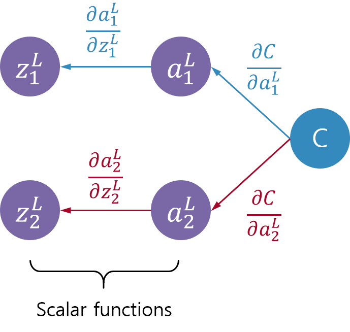
$$ \frac{\partial C}{\partial \mathbf{z}^{L}} = \begin{bmatrix} \dfrac{\partial a^L_1}{\partial z^L_1}\dfrac{\partial C}{\partial a^L_1} + \dfrac{\partial a^L_2}{\partial z^L_1}\dfrac{\partial C}{\partial a^L_2} \\[5pt] \dfrac{\partial a^L_1}{\partial z^L_2}\dfrac{\partial C}{\partial a^L_1} +\dfrac{\partial a^L_2}{\partial z^L_2}\dfrac{\partial C}{\partial a^L_2} \end{bmatrix} \tag{16} $$$\mathbf{z}^L$에 대한 미분이 위와 같은 행렬로 표시되는데 이를 그림으로 알아보면 좀 더 명확하게 의미가 다가 올 수 있다. 네트워크의 마지막 $\mathbf{a}^L$을 출력하는 함수 $f(\mathbf{z}^L)$가 스칼라 함수인 경우와 벡터 함수인 경우로 나눠서 생각해보자. 두 경우에 대해서 네트워크의 마지막 출력과 비용함수는 아래 그림처럼 나타낼 수 있다. 왼쪽이 마지막 활성함수가 스칼라 함수인 경우 (구체적으로는 로지스틱, ReLU 등등)이고 오른쪽이 벡터함수인 경우이다.

앞서도 살펴보았지만 왼쪽 그림처럼 $f \left(\mathbf{z}^L \right)$가 스칼라 함수라면 $z_{1}^L$은 $a_{2}^L$을 계산하는데 관여하지않고 $z_{2}^L$는 $a_{1}^L$을 계산하는데 관여하지 않기 때문에 $\dfrac{\partial a_{2}^L}{\partial z_{1}^L}=0$, $\dfrac{\partial a_{1}^L}{\partial z_{2}^L}=0$이된다. 따라서 식(16) 미분 결과는 다음처럼 간단히 쓸 수 있다.
$$ \frac{\partial C}{\partial \mathbf{z}^{L}} = \begin{bmatrix} \color{#348ABD}{\dfrac{\partial a^L_1}{\partial z^L_1}\dfrac{\partial C}{\partial a^L_1}} \\[5pt] \color{#A60628}{\dfrac{\partial a^L_2}{\partial z^L_2}\dfrac{\partial C}{\partial a^L_2}} \end{bmatrix} \tag{17} $$미분된 결과 행렬의 각 요소를 그림으로 나타내면 아래와 같다. 미분된 각 요소는 아래 그림처럼 색깔로 구분된 경로를 따라 각각 지역미분을 곱하는 과정으로 단순히 연쇄법칙을 적용한 것과 동일하게 된다.
$f(\mathbf{z}^L)$가 소프트맥스처럼 벡터함수였다면 식(16)의 모든 항이 다 값을 가지면서 그대로 아래와 같은 모양이 될 것이다.
$$ \frac{\partial C}{\partial \mathbf{z}^{L}} = \begin{bmatrix} \color{#348ABD}{\dfrac{\partial a^L_1}{\partial z^L_1}\dfrac{\partial C}{\partial a^L_1} + \dfrac{\partial a^L_2}{\partial z^L_1}\dfrac{\partial C}{\partial a^L_2}} \\[5pt] \color{#A60628}{\dfrac{\partial a^L_1}{\partial z^L_2}\dfrac{\partial C}{\partial a^L_1} +\dfrac{\partial a^L_2}{\partial z^L_2}\dfrac{\partial C}{\partial a^L_2}} \end{bmatrix} \tag{18} $$이때 미분한 결과 행렬의 요소를 그림으로 나타내면 아래 그림과 같다.

$\dfrac{\partial C}{\partial z_1^{L}}$은 위 그림에서 왼쪽 경우에 해당하는 것으로 $C$로 부터 $z_1^{L}$로 가는 경로의 미분계수를 경로별로 곱해서 더한 것이다. 그림에서 파란색 경로이며 전체 2개가 있고 각 경로에 대해 연쇄법칙을 적용한 후 이를 더하면 식(18)에 나타난 첫번째 요소가 된다. $\dfrac{\partial C}{\partial z_2^{L}}$는 그림의 오른쪽 경우에 해당하는 것으로 이 역시 그림과 식(18)에 두번째 요소와 일치하는 것을 알 수 있다. 이것으로 야코비안 전치와 그래디언트를 곱하여 유도된 식이 연쇄법칙을 나타내는 그림과도 잘 부합함을 알아보았다.
이제 구체적인 예를 위해 앞서 구해놓은 미분 결과들을 실제로 곱해보도록 하자. 그리고 표기를 간단히 하기위해 비용함수 $C$를 각 층의 가중합 $\mathbf{z}$로 미분한 것, 다시말해 비용함수의 $\mathbf{z}$에 대한 그래디언트를 $\boldsymbol{\delta}$로 두기로 한다.
$$ \boldsymbol{\delta}^L =\frac{\partial C}{\partial \mathbf{z}^{L}} $$1) 비용함수가 제곱합인 경우
제곱합 비용함수의 미분 식(3)과 출력층 활성함수로 로지스틱 함수를 쓴 경우 $\dfrac{\partial \mathbf{a}^L}{\partial \mathbf{z}^L}$인 식(11)을 곱해보자.
$$ \begin{aligned} \boldsymbol{\delta}^L &= \frac{\partial C}{\partial \mathbf{z}^{L}} = \left(\frac{\partial \mathbf{a}^L}{\partial \mathbf{z}^L}\right)^{\text{T}} \frac{\partial C}{\partial \mathbf{a}^L} \\[10pt] &= \begin{bmatrix} a_1^L\left(1-a_1^L\right) & 0 \\[5pt] 0 & a_2^L\left(1-a_2^L\right) \end{bmatrix} \begin{bmatrix} (a^L_1 - y_1) \\[5pt] (a^L_2 - y_2) \end{bmatrix} \\[10pt] &= \begin{bmatrix} a_1^L\left(1-a_1^L\right)(a^L_1 - y_1) \\[5pt] a_2^L\left(1-a_2^L\right)(a^L_2 - y_2) \end{bmatrix} \end{aligned} \tag{19} $$결과는 $\boldsymbol{\delta}^L$의 각 요소가 $a_i^L\left(1-a_i^L\right)(a^L_i - y_i)$꼴이 된다.
여기서 $\mathbf{a}^{L}$을 출력하는 활성함수가 로지스틱, ReLU같은 것들이므로 $\dfrac{\partial \mathbf{a}^L}{\partial \mathbf{z}^L}$가 대각요소만 가지게 된다. 때문에 대각요소만 뽑아내서 $\dfrac{\partial C}{\partial \mathbf{a}^L}$에 엘리먼트 와이즈 곱을 하는 식으로 나타내기도 한다.
$$ \boldsymbol{\delta}^L = \frac{\partial C}{\partial \mathbf{z}^{L}} = \text{diag}\left(\frac{\partial \mathbf{a}^L}{\partial \mathbf{z}^L}\right) \odot \frac{\partial C}{\partial \mathbf{a}^L} $$또는 더 간단하게
$$ \boldsymbol{\delta}^L = \frac{\partial C}{\partial \mathbf{z}^{L}} = \frac{\partial C}{\partial \mathbf{a}^L} \odot \sigma'(\mathbf{z}^L) = \nabla_{\mathbf{a}^{L}} C \odot \sigma'(\mathbf{z}^L) $$로 쓰는 문헌들도 많다.
활성함수가 로지스틱 함수인 경우 $z_i$의 값이 어느정도 크거나 작다면(아래 그림에서 왼쪽으로 -4보다 작거나, 오른쪽으로 4보다 크거나 한 경우) 앞 부분 $a_i^L\left(1-a_i^L\right)$이 거의 0이 되기 때문에 $\delta^L_i$가 점점 0에 가까워지는 포화 현상이 일어나 학습을 더디게 만든다.
 By Qef (Created from scratch with gnuplot) [Public domain], via Wikimedia Commons
식(19) 결과가 맞는지 확인해보자. dz2변수에 결과를 저장하고 비교 해본다.
dmse['dz2'] = np.dot(da2_dz2_logistic.T, dmse['da2'])
dmse['dz2_torch'] = torch.autograd.grad(mse_torch['c'], mse_torch['z2'],
                                        torch.tensor([[1.]]), retain_graph=True)[0]

print(dmse['dz2'])
print(dmse['dz2_torch'])
[[0.1268]
 [0.1451]]
tensor([[0.1268],
        [0.1451]])
2) 비용함수가 바이너리 크로스 엔트로피인 경우
반면 바이너리 크로스엔트로피 비용함수와 로지스틱 함수를 쓴 경우 $\boldsymbol{\delta}^L$을 구해보자. 식(5)와 식(11)을 곱한다.
$$ \begin{aligned} \boldsymbol{\delta}^L &= \frac{\partial C}{\partial \mathbf{z}^{L}} = \left(\frac{\partial \mathbf{a}^L}{\partial \mathbf{z}^L}\right)^{\text{T}} \frac{\partial C}{\partial \mathbf{a}^L} \\[10pt] &= \begin{bmatrix} a_1^L\left(1-a_1^L\right) & 0 \\[5pt] 0 & a_2^L\left(1-a_2^L\right) \end{bmatrix} \begin{bmatrix} -\dfrac{y_1}{a_1^L} + \dfrac{1-y_1}{1-a_1^L} \\[5pt] -\dfrac{y_2}{a_2^L} + \dfrac{1-y_2}{1-a_2^L} \end{bmatrix} \\[10pt] &= \begin{bmatrix} a_1^L\left(1-a_1^L\right)\left(-\dfrac{y_1}{a_1^L} + \dfrac{1-y_1}{1-a_1^L}\right) \\[5pt] a_2^L\left(1-a_2^L\right)\left(-\dfrac{y_2}{a_2^L} + \dfrac{1-y_2}{1-a_2^L}\right) \end{bmatrix} \\[10pt] &= \begin{bmatrix} a_1^L\left(1-a_1^L\right) \left( \dfrac{-y_1\left(1-a_1^L\right) + a_1^L (1-y_1)}{a_1^L\left(1-a_1^L\right)} \right) \\[5pt] a_2^L\left(1-a_2^L\right) \left( \dfrac{-y_2\left(1-a_2^L\right) + a_2^L (1-y_2)}{a_2^L\left(1-a_2^L\right)} \right) \end{bmatrix} \\[10pt] &= \begin{bmatrix} -y_1 + y_1 a^L_1 + a^L_1 - a^L_1 y_1 \\[5pt] -y_2 + y_2 a^L_2 + a^L_2 - a^L_2 y_2 \end{bmatrix} \\[10pt] &= \begin{bmatrix} a^L_1 - y_1 \\[5pt] a^L_2 - y_2 \end{bmatrix} = \mathbf{a}^L - \mathbf{y} \end{aligned} \tag{20} $$앞서 포화를 야기하는 항인 $a_i^L\left(1-a_i^L\right)$부분이 사라지고 $\mathbf{z}$에 대한 그래디언트가 출력과 정답의 단순 차이인 $\boldsymbol{\delta}^L=\mathbf{a}^L - \mathbf{y}$로 깔끔하게 떨어지는 것을 확인할 수 있다. 식(20)을 확인해보자.
dbce['dz2'] = np.dot(da2_dz2_logistic.T, dbce['da2'])
dbce['dz2_torch'] = torch.autograd.grad(bce_torch['c'], bce_torch['z2'],
                                        torch.tensor([[1.]]), retain_graph=True)[0]

print(dbce['dz2'])
print(dbce['dz2_torch'])
[[0.5583]
 [0.7301]]
tensor([[0.5583],
        [0.7301]])
크로스엔트로피 비용함수와 소프트맥스 함수를 쓰는 경우도 이처럼 출력과 정답의 차이가 그래디언트가 되는데 바로 확인해보도록 하자.
3) 비용함수가 크로스 엔트로피인 경우
비용함수가 크로스 엔트로피인 경우 $\dfrac{\partial C}{\partial \mathbf{a}^L}$이 샘플의 정답자리에 의해 식(8), (9)처럼 계산되는 것을 알아 보았다. 만약 원-핫 인코딩된 샘플의 정답이 $\mathbf{y} = [ 1 \quad 0 ]^{\text{T}} $라면 식(8)과 식(12)를 곱한다.
$$ \begin{aligned} \boldsymbol{\delta}^L &= \frac{\partial C}{\partial \mathbf{z}^{L}} = \left(\frac{\partial \mathbf{a}^L}{\partial \mathbf{z}^L}\right)^{\text{T}} \frac{\partial C}{\partial \mathbf{a}^L} \\[10pt] &= \begin{bmatrix} a_1^L\left(1-a_1^L\right) & -a_1^L a_2^L \\[5pt] -a_2^L a_1^L & a_2^L \left(1-a_2^L \right) \end{bmatrix} \begin{bmatrix} - \dfrac{1}{a^L_1} \\[5pt] 0 \end{bmatrix} \\[10pt] &= \begin{bmatrix} a^L_1 - 1 \\ a^L_2 \end{bmatrix} = \begin{bmatrix} a^L_1 \\ a^L_2 \end{bmatrix} - \begin{bmatrix} 1 \\ 0 \end{bmatrix} = \mathbf{a}^{L} - \mathbf{y} \end{aligned} \tag{21} $$만약 원-핫 인코딩된 샘플의 정답이 $\mathbf{y} = [ 0 \quad 1 ]^{\text{T}} $라면 식(9)와 식(12)를 곱한다.
$$ \begin{aligned} \boldsymbol{\delta}^L &= \frac{\partial C}{\partial \mathbf{z}^{L}} = \left(\frac{\partial \mathbf{a}^L}{\partial \mathbf{z}^L}\right)^{\text{T}} \frac{\partial C}{\partial \mathbf{a}^L} \\[10pt] &= \begin{bmatrix} a_1^L\left(1-a_1^L\right) & -a_1^L a_2^L \\[5pt] -a_2^L a_1^L & a_2^L \left(1-a_2^L \right) \end{bmatrix} \begin{bmatrix} 0 \\[5pt] - \dfrac{1}{a^L_2} \end{bmatrix}\\[10pt] &= \begin{bmatrix} a^L_1 \\ a^L_2 - 1 \end{bmatrix} = \begin{bmatrix} a^L_1 \\ a^L_2 \end{bmatrix} - \begin{bmatrix} 0 \\ 1 \end{bmatrix} = \mathbf{a}^{L} - \mathbf{y} \end{aligned} \tag{22} $$타겟이 무엇이든 상관없이 $\boldsymbol{\delta}^L = \mathbf{a}^{L} - \mathbf{y}$라는 결과가 얻어진다.
# 네트워크를 포워드시킬 때 타겟을
# y_bin = np.array([0], dtype=np.long)
# 로 설정했으므로 원-핫 인코딩된 벡터 np.array([1,0])를 출력 a2에서 빼준다.
dce['dz2'] = ce['a2']-np.array([1,0]).reshape(2,1)
dce['dz2_torch'] = torch.autograd.grad(ce_torch['c'], ce_torch['z2'],
                                       torch.tensor([[1.]]), retain_graph=True)[0]

print(dce['dz2'])
print(dce['dz2_torch'])
[[-0.5871]
 [ 0.5871]]
tensor([[-0.5871],
        [ 0.5871]])
식(21), (22)처럼 바로 야코비안 트랜스포즈와 그래디언트를 곱해서 계산해보면 계산 결과는 같음을 알 수 있다.
print( np.dot(da2_dz2_softmax.T, dce['da2']) )
[[-0.5871]
 [ 0.5871]]
5. $\dfrac{\partial C}{\partial \mathbf{b}^{L}}$
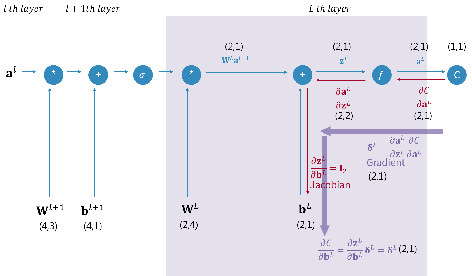
드디어 우리의 목적중 첫번째 파라메터인 $\mathbf{b}^{L}$에 대한 미분을 구할 수 있게 되었다. 역전파 알고리즘에서 구하자고 하는 미분계수는 이 문서에서 보라색으로 표시하고 있다. 위 그림처럼 보라색 화살표를 따라 가면서 미분해놓은 결과를 연쇄법칙에 의해 곱해 나간다. 그렇게 하면 비용함수를 $\mathbf{b}^{L}$로 미분한 결과는 "그래디언트 $\boldsymbol{\delta}^L$과 야코비안 $\dfrac{\partial \mathbf{z}^{L}}{\partial \mathbf{b}^{L}}$의 곱"임을 알 수 있다. 앞서 야코비안은 단위행렬이었으므로 간단히 다음처럼 $\mathbf{b}^{L}$에 대한 미분계수가 구해진다.
$$ \frac{\partial C}{\partial \mathbf{b}^{L}} = \underbrace{\left(\frac{\partial \mathbf{z}^{L}}{\partial \mathbf{b}^{L}}\right)^\text{T}}_{\mathbf{I}} \underbrace{\left(\frac{\partial \mathbf{a}^L}{\partial \mathbf{z}^L}\right)^{\text{T}} \frac{\partial C}{\partial \mathbf{a}^L}}_{\boldsymbol{\delta}^L} = \boldsymbol{\delta}^L \tag{23} $$식(23)에 의해 $\dfrac{\partial C}{\partial \mathbf{b}^{L}}=\boldsymbol{\delta}^L$ 이므로 특별한 계산없이 이전 결과를 그냥 대입한다. 그리고 pytorch로 직접 미분하여 식(23)의 결과를 확인해보자.
dmse['db2'] = dmse['dz2']
dmse['db2_torch'] = torch.autograd.grad(mse_torch['c'], b2_torch,
                                        torch.tensor([[1.]]), retain_graph=True)[0]
print(dmse['db2'])
print(dmse['db2_torch'])
print('\n')

dbce['db2'] = dbce['dz2']
dbce['db2_torch'] = torch.autograd.grad(bce_torch['c'], b2_torch,
                                        torch.tensor([[1.]]), retain_graph=True)[0]
print(dbce['db2'])
print(dbce['db2_torch'])
print('\n')

dce['db2'] = dce['dz2']
dce['db2_torch'] = torch.autograd.grad(ce_torch['c'], b2_torch,
                                       torch.tensor([[1.]]), retain_graph=True)[0]
print(dce['db2'])
print(dce['db2_torch'])
[[0.1268]
 [0.1451]]
tensor([[0.1268],
        [0.1451]])


[[0.5583]
 [0.7301]]
tensor([[0.5583],
        [0.7301]])


[[-0.5871]
 [ 0.5871]]
tensor([[-0.5871],
        [ 0.5871]])
세가지 네트워크 모두에서 손계산한 값과 pytorch로 계산한 값이 일치한다.
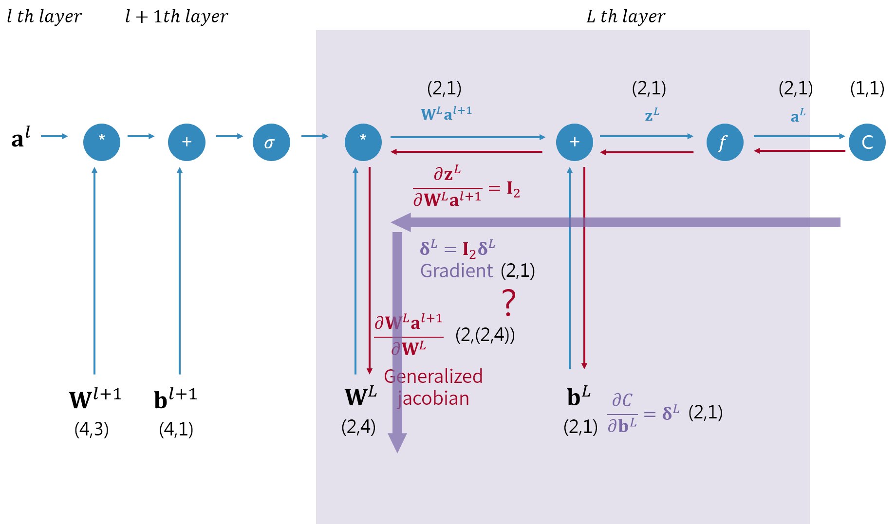
6. $\dfrac{\partial \mathbf{z}^L}{\partial \mathbf{W}^{L}\mathbf{a}^{l+1}} = \dfrac{\partial \mathbf{z}^L}{\partial \mathbf{h}^L} $

$\mathbf{b}^{L}$에 대한 미분을 완성했으므로 이제 $\mathbf{W}^{L}$에 대한 미분을 수행할 차례이다. 먼저 $\mathbf{W}^{L}\mathbf{a}^{l+1}$은 다음과 같다.
$$ \mathbf{W}^{L}\mathbf{a}^{l+1} = \begin{bmatrix} (w^L a^{l+1})_1 \\[5pt] (w^L a^{l+1})_2 \end{bmatrix}= \begin{bmatrix} w^L_{11}a^{l+1}_1 + w^L_{12}a^{l+1}_2 + w^L_{13}a^{l+1}_3 + w^L_{14}a^{l+1}_4 \\[5pt] w^L_{21}a^{l+1}_1 + w^L_{22}a^{l+1}_2 + w^L_{23}a^{l+1}_3 + w^L_{24}a^{l+1}_4 \end{bmatrix} $$그리고 $\mathbf{z}^L$은 다음과 같다.
$$ \mathbf{z}^L = \begin{bmatrix} z^L_1 \\[5pt] z^L_2 \end{bmatrix}=\begin{bmatrix} w^L_{11}a^{l+1}_1 + w^L_{12}a^{l+1}_2 + w^L_{13}a^{l+1}_3 + w^L_{14}a^{l+1}_4 + b^L_1 \\[5pt] w^L_{21}a^{l+1}_1 + w^L_{22}a^{l+1}_2 + w^L_{23}a^{l+1}_3 + w^L_{24}a^{l+1}_4 + b^L_2 \end{bmatrix} = \begin{bmatrix} (w^L a^{l+1})_1 + b^L_1 \\[5pt] (w^L a^{l+1})_2 + b^L_2 \end{bmatrix} $$따라서 구하고자 하는 미분은 다음과 같다.
$$ \begin{aligned} \frac{\partial \mathbf{z}^L}{\partial \mathbf{W}^{L}\mathbf{a}^{l+1}} &= \begin{bmatrix} \dfrac{\partial z^L_1}{\partial (w^L a^{l+1})_1} & \dfrac{\partial z^L_1}{\partial (w^L a^{l+1})_2} \\[5pt] \dfrac{\partial z^L_2}{\partial (w^L a^{l+1})_1} & \dfrac{\partial z^L_2}{\partial (w^L a^{l+1})_2} \end{bmatrix} \\[10pt] &= \begin{bmatrix} \dfrac{\partial (w^L a^{l+1})_1 + b^L_1}{\partial (w^L a^{l+1})_1} & \dfrac{\partial (w^L a^{l+1})_1 + b^L_1}{\partial (w^L a^{l+1})_2} \\[5pt] \dfrac{\partial (w^L a^{l+1})_2 + b^L_2}{\partial (w^L a^{l+1})_1} & \dfrac{\partial (w^L a^{l+1})_2 + b^L_2}{\partial (w^L a^{l+1})_2} \end{bmatrix} \\[10pt] &=\begin{bmatrix} 1 & 0 \\ 0 & 1 \end{bmatrix} \end{aligned} $$결과는 야코비안으로 단위행렬이 된다. 표기를 간략히 하기 위해 $\mathbf{W}^{L}\mathbf{a}^{l+1}=\mathbf{h}^{L}$로 두고 dz2_dh2에 계산결과를 저장하자.
dz2_dh2 = np.eye(2,2)
7. $\dfrac{\partial \mathbf{W}^{L}\mathbf{a}^{l+1}}{\partial \mathbf{W}^L} = \dfrac{\partial \mathbf{h}^{L}}{\partial \mathbf{W}^L}$

이번에 처리할 $\dfrac{\partial \mathbf{W}^{L}\mathbf{a}^{l+1}}{ \partial \mathbf{W}^L}$이 가장 복잡한 부분이다. 왜냐하면 미분하는 변수가 행렬이기 때문이다. 벡터를 벡터로 미분하면 야코비안이 되는데 이 경우는 벡터를 행렬로 미분하기 때문에 약간의 추가 작업이 필요하다. 우선 표기를 간단히 하기위해 좀 전과 같이 $\mathbf{W}^{L}\mathbf{a}^{l+1}$을 $\mathbf{h}^L$로 적기로 하자. 그러면 $\mathbf{h}^L$의 요소인 $h^L_1$, $h^L_2$는 다음과 같다.
$$ \mathbf{h}^L = \begin{bmatrix} h^L_1 \\[5pt] h^L_2 \end{bmatrix}= \begin{bmatrix} w^L_{11}a^{l+1}_1 + w^L_{12}a^{l+1}_2 + w^L_{13}a^{l+1}_3 + w^L_{14}a^{l+1}_4 \\[5pt] w^L_{21}a^{l+1}_1 + w^L_{22}a^{l+1}_2 + w^L_{23}a^{l+1}_3 + w^L_{24}a^{l+1}_4 \end{bmatrix} $$직관적인 방법
그림에도 나타나있듯이 $\mathbf{h}^{L}=\mathbf{W}^{L}\mathbf{a}^{l+1}$은 (2,1)인 벡터이다. 이 벡터를 (2,4)인 행렬로 미분하게 되면 각 벡터 요소 하나를 행렬로 미분하게 되므로 다음처럼 생각해볼 수 있다.

결과는 차원이 (2,2,4)인 다차원 배열이 되는데 딥러닝에서는 이를 텐서라 한다. 이를 일반화된 야코비안generalized jacobian,[Johnson]이라고도 하는데 행이 2이고 그 행의 모양이 (2,4)인 야코비안으로 볼 수 있단 의미이다. 차원을 적어보자면 (2,(2,4))라고 적을 수 있겠다.
우선 이렇게 미분을 마무리하고 다음 단계로 넘어가도록 하자. 이와 관련된 자세한 내용은 9항에서 다시 다루도록 한다.
dh2_dW2 = np.zeros((2,2,4))
dh2_dW2[0,0,:] = mse['a1'].reshape(-1)
dh2_dW2[1,1,:] = mse['a1'].reshape(-1)

print(dh2_dW2)
[[[0.9855 0.9407 0.372  0.943 ]
  [0.     0.     0.     0.    ]]

 [[0.     0.     0.     0.    ]
  [0.9855 0.9407 0.372  0.943 ]]]
vec 연산자를 이용[임성빈]

수학적으로 노테이션을 좀 더 완전하게 하려면 $\mathbf{W}^L$행렬에 $\text{vec}()$연산자를 취해 벡터로 만들어서 미분하는 방식을 선택할 수 있다. $\text{vec}()$연산자를 취하는 것은 행렬을 (2)전치 시키는 것과 같다.
$$ \text{vec}\left(\mathbf{W}^L\right) = \left(\mathbf{W}^L\right)^{(2)} = \begin{bmatrix} w^L_{11} \\[5pt] w^L_{21} \\[5pt] w^L_{12} \\[5pt] w^L_{22} \\[5pt] w^L_{13} \\[5pt] w^L_{23} \\[5pt] w^L_{14} \\[5pt] w^L_{24} \end{bmatrix} $$이처럼 미분하는 행렬을 벡터로 만들어 벡터 $\mathbf{h}^{L}$을 벡터 $\text{vec}\left(\mathbf{W}^L\right)$로 분모 레이아웃 방식으로 미분한다.
$$ \frac{\partial \mathbf{h}^{L}}{\partial \mathbf{W}^L} = \frac{\partial \mathbf{h}^{L}}{\partial \text{vec}(\mathbf{W}^L)}= \begin{bmatrix} \dfrac{\partial h_1}{\partial w^L_{11}} & \dfrac{\partial h_2}{\partial w^L_{11}} \\[5pt] \dfrac{\partial h_1}{\partial w^L_{21}} & \dfrac{\partial h_2}{\partial w^L_{21}} \\[5pt] \dfrac{\partial h_1}{\partial w^L_{12}} & \dfrac{\partial h_2}{\partial w^L_{12}} \\[5pt] \dfrac{\partial h_1}{\partial w^L_{22}} & \dfrac{\partial h_2}{\partial w^L_{22}} \\[5pt] \dfrac{\partial h_1}{\partial w^L_{13}} & \dfrac{\partial h_2}{\partial w^L_{13}} \\[5pt] \dfrac{\partial h_1}{\partial w^L_{23}} & \dfrac{\partial h_2}{\partial w^L_{23}} \\[5pt] \dfrac{\partial h_1}{\partial w^L_{14}} & \dfrac{\partial h_2}{\partial w^L_{14}} \\[5pt] \dfrac{\partial h_1}{\partial w^L_{24}} & \dfrac{\partial h_2}{\partial w^L_{24}} \end{bmatrix} = \begin{bmatrix} a^{l+1}_1 & 0 \\[5pt] 0 & a^{l+1}_1 \\[5pt] a^{l+1}_2 & 0 \\[5pt] 0 & a^{l+1}_2 \\[5pt] a^{l+1}_3 & 0 \\[5pt] 0 & a^{l+1}_3 \\[5pt] a^{l+1}_4 & 0 \\[5pt] 0 & a^{l+1}_4 \end{bmatrix} = \begin{bmatrix} a^{l+1}_1 \mathbf{I}_2 \\[10pt] a^{l+1}_2 \mathbf{I}_2 \\[10pt] a^{l+1}_3 \mathbf{I}_2 \\[10pt] a^{l+1}_4 \mathbf{I}_2 \end{bmatrix} = \mathbf{a}^{l+1} \otimes \mathbf{I} \tag{24} $$이 과정으로 미분을 하면 분모 레이아웃으로 미분했으므로 전치된 야코비안을 얻게 된다. 식(24)의 마지막 과정은 행렬을 간략하게 나타내기 위해 크로네커곱 연산자 $\otimes$를 도입하여 적은것이다.
numpy에서 크로네커 곱 연산자를 지원하지 않으므로 np.tile, np.repeat함수를 이용해 식(24)를 구현해둔다.
dh2_dvecW2 = np.tile(np.eye(2,2), (4,1))*np.repeat(mse['a1'], 2, axis=0)

print(dh2_dvecW2)
[[0.9855 0.    ]
 [0.     0.9855]
 [0.9407 0.    ]
 [0.     0.9407]
 [0.372  0.    ]
 [0.     0.372 ]
 [0.943  0.    ]
 [0.     0.943 ]]
8. $\dfrac{\partial C}{\partial \mathbf{w}^{L}\mathbf{a}^{l+1}} = \dfrac{\partial \mathbf{z}^L}{\partial \mathbf{w}^{L}\mathbf{a}^{l+1}} \boldsymbol{\delta}^L$
이제 $\mathbf{W}^{L}$에 대한 미분을 완성하기 위해서 지역 미분들을 연쇄법칙에 의해 차례대로 곱해 나간다.

현재까지 누적시켜온 그래디언트 $\boldsymbol{\delta}^L$과 $\dfrac{\partial \mathbf{z}^L}{\partial \mathbf{W}^{L}\mathbf{a}^{l+1}}$을 곱한다. 곱해지는 행렬의 크기를 보면 (2,2)(2,1) = (2,1)으로 차원이 잘 맞는 것을 알 수 있다.
$$ \frac{\partial \mathbf{z}^L}{\partial \mathbf{W}^{L}\mathbf{a}^{l+1}} \boldsymbol{\delta}^L = \mathbf{I}_2 \boldsymbol{\delta}^L= \boldsymbol{\delta}^L $$$\mathbf{W}^L$로 미분하기 직전까지 미분한 그래디언트는 여전히 $\boldsymbol{\delta}^L$이다.
아래 코드로 현재까지 미분을 저장해둔다.
dmse['dh2'] = np.dot(dz2_dh2, dmse['dz2'])
dbce['dh2'] = np.dot(dz2_dh2, dbce['dz2'])
dce['dh2']  = np.dot(dz2_dh2, dce['dz2'])
9. $\dfrac{\partial C}{\partial \mathbf{W}^{L}}$
이제 우리의 목적 중 두번째 파라메터인 $\mathbf{W}^{L}$에 대한 미분도 구할 수 있게 되었다. Deep learning[Goodfellow et. al.]에서도 역전파 알고리즘을 다음과 같이 밝히고 있다.
In this rearranged view, back-propagation is still just multiplying Jacobians by gradients. p.203
따라서 비용함수를 $\mathbf{W}^{L}$로 미분한 결과는 5항에서 $\mathbf{b}^{L}$로 미분할 때와 마찬가지로 여전히 "그래디언트 $\boldsymbol{\delta}^L$과 야코비안 전치의 곱"이 되어야 한다.
7항에서 $\dfrac{\partial \mathbf{W}^{L}\mathbf{a}^{l+1}}{ \partial \mathbf{W}^L}$를 계산할 때 직관적인 방법과 vec연산자를 이용하는 방법 두가지로 계산을 했었다. 이 두가지 경우에 대해서 모두 "그래디언트와 야코비안 전치의 곱"으로 계산되는지 알아보도록 하자.
직관적인 방법
7항에서 구한 $\dfrac{\partial \mathbf{W}^{L}\mathbf{a}^{l+1}}{ \partial \mathbf{W}^L}$와 8항에서 구한 $\boldsymbol{\delta}^L$를 위 그림처럼 곱하면 원하는 미분이 구해져야 한다. 곱을 하기 위해 차원을 확인해보면 각 차원은 (2,(2,4)), (2,1)이다. 그래서 이 둘을 단순히 행렬곱할 수 없다는 것을 알 수 있다.

이 둘의 곱을 수행하고 그것이 어떤 의미를 가지는 알아보기위해 위 그림을 보기로 하자. 위 그림은 이 글 처음에 제시한 네트워크 그림과 약간 다른데 $\mathbf{W}^{L}\mathbf{a}^{l+1}$을 $\mathbf{h}^{L}$로 두어 더 세분화 하여 그린것이다. 그림을 보면 비용 함수 $C$에 대한 $\mathbf{W}^L$의 미분은 연쇄법칙을 통해 파란색 경로를 따라 곱한 미분과 빨간색 경로를 따라 곱한 미분을 더한 것이라는 것을 알 수 있다. 식으로 쓰면 다음과 같다.
$$ \frac{\partial C}{\partial \mathbf{W}^L} = \color{#348ABD}{\frac{\partial h_1^L}{\partial \mathbf{W}^L}\frac{\partial C}{\partial h^L_1}} + \color{#A60628}{\frac{\partial h_2^L}{\partial \mathbf{W}^L}\frac{\partial C}{\partial h^L_2}} $$식에 나타난 $\dfrac{\partial h_1^L}{\partial \mathbf{W}^L}$, $\dfrac{\partial h_2^L}{\partial \mathbf{W}^L}$은 7항에서 계산했고, $\dfrac{\partial C}{\partial h^L_1}$, $\dfrac{\partial C}{\partial h^L_2}$은 8항에서 이미 모두 계산해 놓은 것들이다. 8항에 의해 $\dfrac{\partial C}{\partial \mathbf{h}^L}=\boldsymbol{\delta}$이다. 이미 계산해놓은 일반화된 야코비안과 그래디언트 $\boldsymbol{\delta}^L$를 이용해 위 식대로 계산하는 것은 아래 그림처럼 계산하는 것과 같다.

그림은 일반회된 야코비안의 각 행에 $\boldsymbol{\delta}^L$의 각 요소를 곱하고 나서 행을 모두 더하는 것을 설명하고 있다. 여기서 일반화된 야코비안의 각 행이란 위 그림의 파란색, 빨간색 행렬을 의미한다. 이제 각 경우에 대해서 단계적으로 계산을 해보자. 우선 일반화된 야코비안의 첫행과 둘째행을 각각 적어보면 다음과 같다.
$$ \begin{aligned} \frac{\partial h_1^L}{\partial \mathbf{W}^L}&=\begin{bmatrix} a^{l+1}_1 & a^{l+1}_2 & a^{l+1}_3 & a^{l+1}_4 \\ 0 & 0 & 0 & 0 \end{bmatrix} \\[10pt] \frac{\partial h_2^L}{\partial \mathbf{W}^L}&=\begin{bmatrix} 0 & 0 & 0 & 0 \\ a^{l+1}_1 & a^{l+1}_2 & a^{l+1}_3 & a^{l+1}_4 \end{bmatrix} \end{aligned} $$이 둘에 $\delta^L_1$과 $\delta^L_2$를 각각 곱한다.
$$ \color{#348ABD}{\frac{\partial h_1^L}{\partial \mathbf{W}^L}\frac{\partial C}{\partial h^L_1}}= \begin{bmatrix} a^{l+1}_1 \delta^L_1 & a^{l+1}_2 \delta^L_1 & a^{l+1}_3 \delta^L_1 & a^{l+1}_4 \delta^L_1 \\ 0 & 0 & 0 & 0 \end{bmatrix} $$$$ \color{#A60628}{\frac{\partial h_2^L}{\partial \mathbf{W}^L}\frac{\partial C}{\partial h^L_2}} = \begin{bmatrix} 0 & 0 & 0 & 0 \\ a^{l+1}_1 \delta^L_2 & a^{l+1}_2 \delta^L_2 & a^{l+1}_3 \delta^L_2 & a^{l+1}_4 \delta^L_2 \end{bmatrix} $$그리고 이 둘을 더하면 다음처럼 $\mathbf{W}^L$에 대한 미분이 간단히 완성된다.
$$ \begin{aligned} \frac{\partial C}{\partial \mathbf{W}^L} &= \color{#348ABD}{\frac{\partial h_1^L}{\partial \mathbf{W}^L}\frac{\partial C}{\partial h^L_1}} + \color{#A60628}{\frac{\partial h_2^L}{\partial \mathbf{W}^L}\frac{\partial C}{\partial h^L_2}} \\[10pt] &= \begin{bmatrix} a^{l+1}_1 \delta^L_1 & a^{l+1}_2 \delta^L_1 & a^{l+1}_3 \delta^L_1 & a^{l+1}_4 \delta^L_1 \\ a^{l+1}_1 \delta^L_2 & a^{l+1}_2 \delta^L_2 & a^{l+1}_3 \delta^L_2 & a^{l+1}_4 \delta^L_2 \end{bmatrix} \\[10pt] &= \boldsymbol{\delta}^L \left(\mathbf{a}^{l+1}\right)^{\text{T}} \end{aligned} \tag{25} $$numpy의 브로드캐스팅을 이용하여 위 곱의 합을 구현해서 pytorch로 미분한 결과와 비교해보자.
print( (dh2_dW2 * dmse['dh2']).sum(axis=0) )
dmse['dW2_torch'] = torch.autograd.grad(mse_torch['c'], W2_torch,
                                        torch.tensor([[1.]]), retain_graph=True)[0]
print(dmse['dW2_torch'])
print('\n')

print( (dh2_dW2 * dbce['dh2']).sum(axis=0) )
dbce['dW2_torch'] = torch.autograd.grad(bce_torch['c'], W2_torch,
                                        torch.tensor([[1.]]), retain_graph=True)[0]
print(dbce['dW2_torch'])
print('\n')

print( (dh2_dW2 * dce['dh2']).sum(axis=0) )
dce['dW2_torch'] = torch.autograd.grad(ce_torch['c'], W2_torch,
                                       torch.tensor([[1.]]), retain_graph=True)[0]
print(dce['dW2_torch'])
[[0.125  0.1193 0.0472 0.1196]
 [0.143  0.1365 0.054  0.1368]]
tensor([[0.1250, 0.1193, 0.0472, 0.1196],
        [0.1430, 0.1365, 0.0540, 0.1368]])


[[0.5502 0.5252 0.2077 0.5264]
 [0.7195 0.6868 0.2716 0.6884]]
tensor([[0.5502, 0.5252, 0.2077, 0.5264],
        [0.7195, 0.6868, 0.2716, 0.6884]])


[[-0.5786 -0.5523 -0.2184 -0.5536]
 [ 0.5786  0.5523  0.2184  0.5536]]
tensor([[-0.5786, -0.5523, -0.2184, -0.5536],
        [ 0.5786,  0.5523,  0.2184,  0.5536]])
세 네트워크 모두에서 결과가 같다. 복잡하게 하지말고 식(25)에서 정리된 결과로 바로 계산해도 계산 결과는 같다.
$$ \frac{\partial C}{\partial \mathbf{W}^L} = \boldsymbol{\delta}^L \left(\mathbf{a}^{l+1}\right)^{\text{T}} $$dmse['dW2'] = dmse['dh2']*mse['a1'].T
print( dmse['dW2'] )
print('\n')
dbce['dW2'] = dbce['dh2']*bce['a1'].T
print( dbce['dW2'] )
print('\n')
dce['dW2'] = dce['dh2']*ce['a1'].T
print( dce['dW2'] )
[[0.125  0.1193 0.0472 0.1196]
 [0.143  0.1365 0.054  0.1368]]


[[0.5502 0.5252 0.2077 0.5264]
 [0.7195 0.6868 0.2716 0.6884]]


[[-0.5786 -0.5523 -0.2184 -0.5536]
 [ 0.5786  0.5523  0.2184  0.5536]]
역시 결과는 동일하다.
다변수 함수의 연쇄법칙을 이용해서 위 절차대로 $\mathbf{W}^L$에 대한 미분을 완성했지만 여기에는 한가지 문제가 있다. 위 과정은 더이상 야코비안 전치와 그래디언트를 곱하는 과정이 아니다. 야코비안 전치 조차도 나온적이 없다. 이 과정을 야코비안 전치와 그래디언트의 곱으로 만들기 위해 행렬을 벡터로 펼쳐주는 과정이 필요하다. Deep learning에서 이 과정을 다음과 같이 설명하고 있다.
The only difference is how the numbers are arranged in a grid to form a tensor. We could imagine flattening each tensor into
a vector before we run back-propagation, computing a vector-valued gradient, and then reshaping the gradient back into a tensor. p.203
일반화된 야코비안에도 '야코비안 전치와 그래디언트 곱'이라는 규칙을 적용하기 위해 위 인용된 과정을 수행해보자. 절차대로 진행하기 위해 가장 먼저 야코비안을 전치시킨다. (2,(2,4))를 ((2,4),2)로 만든다. 아래 그림처럼 전치된다.
전치시킨 상태에서도 그래디언트와 곱을 할 수 없으므로 ((2,4),2)를 (8,2)로 만든다. 이 과정을 flattening이라 한다.

이제 그래디언트와 곱한다.
계산 과정에서 전치, flattening 했으므로 이번에는 결과를 flattening 역과정, 전치를 해서 원래대로 되돌린다. 먼저 flattening의 역과정을 적용한 다음
$$ \begin{bmatrix} a^{l+1}_1 \delta^L_1 \\[5pt] a^{l+1}_2 \delta^L_1 \\[5pt] a^{l+1}_3 \delta^L_1 \\[5pt] a^{l+1}_4 \delta^L_1 \\[5pt] a^{l+1}_1 \delta^L_2 \\[5pt] a^{l+1}_2 \delta^L_2 \\[5pt] a^{l+1}_3 \delta^L_2 \\[5pt] a^{l+1}_4 \delta^L_2 \\ \end{bmatrix} = \begin{bmatrix} a^{l+1}_1 \delta^L_1 & a^{l+1}_1 \delta^L_2 \\[5pt] a^{l+1}_2 \delta^L_1 & a^{l+1}_2 \delta^L_2 \\[5pt] a^{l+1}_3 \delta^L_1 & a^{l+1}_3 \delta^L_2 \\[5pt] a^{l+1}_4 \delta^L_1 & a^{l+1}_4 \delta^L_2 \end{bmatrix} $$이제 전치시키면 식(25)와 동일한 결과를 얻을 수 있다.
$$ \begin{bmatrix} a^{l+1}_1 \delta^L_1 & a^{l+1}_1 \delta^L_2 \\[5pt] a^{l+1}_2 \delta^L_1 & a^{l+1}_2 \delta^L_2 \\[5pt] a^{l+1}_3 \delta^L_1 & a^{l+1}_3 \delta^L_2 \\[5pt] a^{l+1}_4 \delta^L_1 & a^{l+1}_4 \delta^L_2 \end{bmatrix}^\text{T}= \begin{bmatrix} a^{l+1}_1 \delta^L_1 & a^{l+1}_2 \delta^L_1 & a^{l+1}_3 \delta^L_1 & a^{l+1}_4 \delta^L_1 \\[5pt] a^{l+1}_1 \delta^L_2 & a^{l+1}_2 \delta^L_2 & a^{l+1}_3 \delta^L_2 & a^{l+1}_4 \delta^L_2 \end{bmatrix} = \boldsymbol{\delta}^L \left(\mathbf{a}^{l+1}\right)^{\text{T}} $$vec 연산자를 이용한 방법
이번에는 vec 연산자를 사용한 방법으로 같은 결과를 얻을 수 있는지 알아본다.

여기서는 $\mathbf{W}^L$에 vec 연산자를 적용하여 $\mathbf{W}^L$을 (8,1) 열벡터로 변환하여 분모 레이아웃으로 미분을 하였다. 그 결과로 (8,2)인 전치된 야코비안을 얻을 수 있었다. 그렇기 때문에 "그래디언트와 야코비안 전치의 곱"이란 룰에 의해 그냥 바로 곱할 수 있다.
$$ \frac{\partial \mathbf{W}^{L}\mathbf{a}^{l+1}}{\partial \text{vec}\left(\mathbf{W}^L\right)} \boldsymbol{\delta}^L = \begin{bmatrix} a^{l+1}_1 & 0 \\[5pt] 0 & a^{l+1}_1 \\[5pt] a^{l+1}_2 & 0 \\[5pt] 0 & a^{l+1}_2 \\[5pt] a^{l+1}_3 & 0 \\[5pt] 0 & a^{l+1}_3 \\[5pt] a^{l+1}_4 & 0 \\[5pt] 0 & a^{l+1}_4 \end{bmatrix} \begin{bmatrix} \delta^L_1 \\[10pt] \delta^L_2 \end{bmatrix} = \begin{bmatrix} a^{l+1}_1\delta^L_1 \\[5pt] a^{l+1}_1\delta^L_2 \\[5pt] a^{l+1}_2\delta^L_1 \\[5pt] a^{l+1}_2\delta^L_2 \\[5pt] a^{l+1}_3\delta^L_1 \\[5pt] a^{l+1}_3\delta^L_2 \\[5pt] a^{l+1}_4\delta^L_1 \\[5pt] a^{l+1}_4\delta^L_2 \end{bmatrix} $$이 결과는 $\mathbf{W}^L$에 vec 연산자를 취한 후 다르게 말하면 (2)전치 시킨 후 미분한 결과이다. 따라서 원래 결과로 돌려놓기 위해 결과를 (2)전치시킨다.
$$ \begin{bmatrix} a^{l+1}_1\delta^L_1 \\[5pt] a^{l+1}_1\delta^L_2 \\[5pt] a^{l+1}_2\delta^L_1 \\[5pt] a^{l+1}_2\delta^L_2 \\[5pt] a^{l+1}_3\delta^L_1 \\[5pt] a^{l+1}_3\delta^L_2 \\[5pt] a^{l+1}_4\delta^L_1 \\[5pt] a^{l+1}_4\delta^L_2 \end{bmatrix}^{(2)} = \begin{bmatrix} a^{l+1}_1 \delta^L_1 & a^{l+1}_2 \delta^L_1 & a^{l+1}_3 \delta^L_1 & a^{l+1}_4 \delta^L_1 \\[5pt] a^{l+1}_1 \delta^L_2 & a^{l+1}_2 \delta^L_2 & a^{l+1}_3 \delta^L_2 & a^{l+1}_4 \delta^L_2 \end{bmatrix} = \boldsymbol{\delta}^L \left(\mathbf{a}^{l+1}\right)^{\text{T}} $$이전과 동일한 결과를 얻을 수 있다. 이 방법은 vec 연산자와 vec 전치같은 생소한 개념이 나오기는 하지만 계산 과정은 훨씬 간편하다는 것을 알 수 있다.
이 과정을 python으로 코딩하고 이미 계산해둔 dW2와 비교해보자. 마지막 (8,1)을 (2,4)로 (2)전치시키는 과정에서 그냥 reshape(2,4)를 하면 행우선 방식으로 진행되므로 FORTRAN 스타일인 열우선 방식으로 진행하기 위해서 order="F"옵션을 준다.
# (2)전치를 위해 reshape(2, 4, order="F") 한다.

print(np.dot(dh2_dvecW2, dmse['dh2']).reshape(2, 4, order="F"))
print(dmse['dW2'])
print('\n')

print(np.dot(dh2_dvecW2, dbce['dh2']).reshape(2, 4, order="F"))
print(dbce['dW2'])
print('\n')

print(np.dot(dh2_dvecW2, dce['dh2']).reshape(2, 4, order="F"))
print(dce['dW2'])
[[0.125  0.1193 0.0472 0.1196]
 [0.143  0.1365 0.054  0.1368]]
[[0.125  0.1193 0.0472 0.1196]
 [0.143  0.1365 0.054  0.1368]]


[[0.5502 0.5252 0.2077 0.5264]
 [0.7195 0.6868 0.2716 0.6884]]
[[0.5502 0.5252 0.2077 0.5264]
 [0.7195 0.6868 0.2716 0.6884]]


[[-0.5786 -0.5523 -0.2184 -0.5536]
 [ 0.5786  0.5523  0.2184  0.5536]]
[[-0.5786 -0.5523 -0.2184 -0.5536]
 [ 0.5786  0.5523  0.2184  0.5536]]
결과는 모두 같다.
이것으로 $L$층에 대한 미분이 모두 끝냈다. $l+1$층에 대한 미분도 이 과정과 완전히 동일하게 진행된다.
10. $\dfrac{\partial \mathbf{W}^{L}\mathbf{a}^{l+1}}{\partial \mathbf{a}^{l+1}}$

지금부터는 이전과 마찬가지로 같은 내용이 반복된다.
$$ \mathbf{W}^{L}\mathbf{a}^{l+1} = \begin{bmatrix} w_{11}^L a^{l+1}_1 + w_{12}^L a^{l+1}_2 + w_{13}^L a^{l+1}_3 + w_{14}^L a^{l+1}_4 \\ w_{21}^L a^{l+1}_1 + w_{22}^L a^{l+1}_2 + w_{23}^L a^{l+1}_3 + w_{24}^L a^{l+1}_4 \end{bmatrix} $$이고 이것을 $\mathbf{a}^{l+1}$로 미분하면 다음과 같다.
$$ \begin{aligned} \frac{\partial \mathbf{W}^{L}\mathbf{a}^{l+1}}{\partial \mathbf{a}^{l+1}} &= \begin{bmatrix} \dfrac{\partial (\mathbf{W}^{L}\mathbf{a}^{l+1})_{1} }{ \partial a^{l+1}_1 } & \dfrac{\partial (\mathbf{W}^{L}\mathbf{a}^{l+1})_{1} }{ \partial a^{l+1}_2 } & \dfrac{\partial (\mathbf{W}^{L}\mathbf{a}^{l+1})_{1} }{ \partial a^{l+1}_3 } & \dfrac{\partial (\mathbf{W}^{L}\mathbf{a}^{l+1})_{1} }{ \partial a^{l+1}_4 } \\ \dfrac{\partial (\mathbf{W}^{L}\mathbf{a}^{l+1})_{2} }{ \partial a^{l+1}_1 } & \dfrac{\partial (\mathbf{W}^{L}\mathbf{a}^{l+1})_{2} }{ \partial a^{l+1}_2 } & \dfrac{\partial (\mathbf{W}^{L}\mathbf{a}^{l+1})_{2} }{ \partial a^{l+1}_3 } & \dfrac{\partial (\mathbf{W}^{L}\mathbf{a}^{l+1})_{2} }{ \partial a^{l+1}_4 } \end{bmatrix} \\[10pt] &=\begin{bmatrix} w_{11}^L & w_{12}^L & w_{13}^L & w_{14}^L \\ w_{21}^L & w_{22}^L & w_{23}^L & w_{24}^L \end{bmatrix} \\[10pt] &= \mathbf{W}^{L} \end{aligned} $$간단하게 다음처럼 야코비안을 저장해둔다.
dh2_da1 = W2

print(dh2_da1)
[[0.8929 0.2135 0.1067 0.4187]
 [0.6669 0.9168 0.1205 0.2631]]
11. $\dfrac{\partial \mathbf{a}^{l+1}}{\partial \mathbf{z}^{l+1}}$

$l+1$층에 대한 미분은 야코비안 $\dfrac{\partial \mathbf{a}^{l+1}}{\partial \mathbf{z}^{l+1}}$을 구하는 것으로 시작한다. 우선 야코비안을 적어보면 다음과 같다.
$$ \frac{\partial \mathbf{a}^{l+1}}{\partial \mathbf{z}^{l+1}} = \begin{bmatrix} \dfrac{\partial a^{l+1}_1}{\partial z^{l+1}_1} & \dfrac{\partial a^{l+1}_1}{\partial z^{l+1}_2} & \dfrac{\partial a^{l+1}_1}{\partial z^{l+1}_3} & \dfrac{\partial a^{l+1}_1}{\partial z^{l+1}_4} \\ \dfrac{\partial a^{l+1}_2}{\partial z^{l+1}_1} & \dfrac{\partial a^{l+1}_2}{\partial z^{l+1}_2} & \dfrac{\partial a^{l+1}_2}{\partial z^{l+1}_3} & \dfrac{\partial a^{l+1}_2}{\partial z^{l+1}_4} \\ \dfrac{\partial a^{l+1}_3}{\partial z^{l+1}_1} & \dfrac{\partial a^{l+1}_3}{\partial z^{l+1}_2} & \dfrac{\partial a^{l+1}_3}{\partial z^{l+1}_3} & \dfrac{\partial a^{l+1}_3}{\partial z^{l+1}_4} \\ \dfrac{\partial a^{l+1}_4}{\partial z^{l+1}_1} & \dfrac{\partial a^{l+1}_4}{\partial z^{l+1}_2} & \dfrac{\partial a^{l+1}_4}{\partial z^{l+1}_3} & \dfrac{\partial a^{l+1}_4}{\partial z^{l+1}_4} \end{bmatrix} $$그런데 활성함수는 일변수 스칼라 함수이므로 대각요소를 제외하면 모두 0이 된다. 이는 식(11)에서 이미 알아본 바이다. $\mathbf{z}^{l+1}$을 입력받는 활성함수를 미분해야 하는데 여기서 활성함수는 로지스틱 시그모이드 함수로 가정을 한다. 그러면 $\dfrac{\partial \mathbf{a}^{l+1}}{\partial \mathbf{z}^{l+1}}$은 다음처럼 된다.
$$ \frac{\partial \mathbf{a}^{l+1}}{\partial \mathbf{z}^{l+1}} = \begin{bmatrix} a^{l+1}_1(1-a^{l+1}_1) & 0 & 0 & 0 \\ 0 & a^{l+1}_2(1-a^{l+1}_2) & 0 & 0 \\ 0 & 0 & a^{l+1}_3(1-a^{l+1}_3) & 0 \\ 0 & 0 & 0 & a^{l+1}_4(1-a^{l+1}_4) \end{bmatrix} $$식(11)을 구현한 코드와 동일한 코드로 야코비안 $\dfrac{\partial \mathbf{a}^{l+1}}{\partial \mathbf{z}^{l+1}}$을 준비해둔다.
da1_dz1 = np.eye(4,4)
da1_dz1 = da1_dz1 * logistic_prime(mse['z1'])
print(da1_dz1)
[[0.0143 0.     0.     0.    ]
 [0.     0.0558 0.     0.    ]
 [0.     0.     0.2336 0.    ]
 [0.     0.     0.     0.0538]]
12. $\dfrac{\partial \mathbf{z}^{l+1}}{\partial \mathbf{b}^{l+1}}$

야코비안 $\dfrac{\partial \mathbf{z}^{l+1}}{\partial \mathbf{b}^{l+1}}$는 이전 과정에서 알아봤듯이 4$\times$4 단위행렬이 된다.
dz1_db1 = np.eye(4,4)
13. $\dfrac{\partial C}{\partial \mathbf{a}^{l+1}}$

이제 미분해놓은 미분 계수들을 차례대로 곱하면서 $\mathbf{b}^{l+1}$에 대한 미분을 구할 때 까지 진행한다. $\dfrac{\partial C}{\partial \mathbf{a}^{l+1}}$를 구하기 위해 다음 식처럼 연쇄법칙을 적용한다.
$$ \frac{\partial C}{\partial \mathbf{a}^{l+1}} = \left(\frac{\partial \mathbf{W}^L \mathbf{a}^{l+1}}{\partial \mathbf{a}^{l+1}} \right)^\text{T} \boldsymbol{\delta}^L $$$\dfrac{\partial \mathbf{W}^L \mathbf{a}^{l+1}}{\partial \mathbf{a}^{l+1}}$는 10번 과정을 통해 $\mathbf{W}^L$이므로 결국 다음과 같이 된다.
$$ \frac{\partial C}{\partial \mathbf{a}^{l+1}} = \left(\mathbf{W}^L \right)^\text{T} \boldsymbol{\delta}^L \tag{26} $$이제 $\mathbf{a}^{l+1}$미분한 그래디언트를 코드로 계산해보자. 특별한 것은 없고 지금까지 해오던것처럼 식(26)을 직접 계산한것과 pytorch로 구한 그래디언트를 비교해본다.
# 'dz2'변수에 delta^L이 저장되어 있음 delta는 z로 미분한 미분계수임을 상기할 것
dmse['da1'] = np.dot(dh2_da1.T, dmse['dz2'])
dmse['da1_torch'] = torch.autograd.grad(mse_torch['c'],  mse_torch['a1'],
                                        torch.tensor([[1.]]), retain_graph=True)[0]
print(dmse['da1'])
print(dmse['da1_torch'])
print('\n')

dbce['da1'] = np.dot(dh2_da1.T, dbce['dz2'])
dbce['da1_torch'] = torch.autograd.grad(bce_torch['c'],  bce_torch['a1'],
                                        torch.tensor([[1.]]), retain_graph=True)[0]
print(dbce['da1'])
print(dbce['da1_torch'])
print('\n')

dce['da1'] = np.dot(dh2_da1.T, dce['dz2'])
dce['da1_torch'] = torch.autograd.grad(ce_torch['c'],  ce_torch['a1'],
                                       torch.tensor([[1.]]), retain_graph=True)[0]
print(dce['da1'])
print(dce['da1_torch'])
[[0.21  ]
 [0.1601]
 [0.031 ]
 [0.0913]]
tensor([[0.2100],
        [0.1601],
        [0.0310],
        [0.0913]])


[[0.9853]
 [0.7885]
 [0.1475]
 [0.4258]]
tensor([[0.9853],
        [0.7885],
        [0.1475],
        [0.4258]])


[[-0.1327]
 [ 0.4129]
 [ 0.0081]
 [-0.0913]]
tensor([[-0.1327],
        [ 0.4129],
        [ 0.0081],
        [-0.0913]])
이번에도 모든 네트워크에 대해서 그래디언트 값이 동일한 것을 알 수 있다.
14. $\dfrac{\partial C}{\partial \mathbf{z}^{l+1}}$

이제 $\dfrac{\partial C}{\partial \mathbf{z}^{l+1}}$을 구할 차례다 이 미분 계수를 구한 다음 결과를 $L$층에서도 그렇게 했듯이 $\boldsymbol{\delta}^{l+1}$로 두기로 하자. (각 층의 가중합 $\mathbf{z}$에 대한 미분을 $\boldsymbol{\delta}$로 두고 있다.) 구하고자 하는 미분은 연쇄법칙에 의해 다음과 같다.
$$ \frac{\partial C}{\partial \mathbf{z}^{l+1}}=\left(\frac{\partial \mathbf{a}^{l+1}}{\partial \mathbf{z}^{l+1}}\right)^{\text{T}}\frac{\partial C}{\partial \mathbf{a}^{l+1}} $$우변에 각항은 이미 모두 구해 놓았다. $\dfrac{\partial \mathbf{a}^{l+1}}{\partial \mathbf{z}^{l+1}}$은 11번 과정에 의해 유도되어 da1_dz1변수에 저장되어있다. $\dfrac{\partial C}{\partial \mathbf{a}^{l+1}}$는 방금 13번 과정을 통해 구하였다. 이 둘을 단지 곱하기만 하면 $\boldsymbol{\delta}^{l+1}$을 구할 수 있다.
dmse['dz1'] = np.dot(da1_dz1.T, dmse['da1'])
dmse['dz1_torch'] = torch.autograd.grad(mse_torch['c'],  mse_torch['z1'],
                                        torch.tensor([[1.]]), retain_graph=True)[0]
print(dmse['dz1'])
print(dmse['dz1_torch'])
print('\n')

dbce['dz1'] = np.dot(da1_dz1.T, dbce['da1'])
dbce['dz1_torch'] = torch.autograd.grad(bce_torch['c'],  bce_torch['z1'],
                                        torch.tensor([[1.]]), retain_graph=True)[0]
print(dbce['dz1'])
print(dbce['dz1_torch'])
print('\n')

dce['dz1'] = np.dot(da1_dz1.T, dce['da1'])
dce['dz1_torch'] = torch.autograd.grad(ce_torch['c'],  ce_torch['z1'],
                                       torch.tensor([[1.]]), retain_graph=True)[0]
print(dce['dz1'])
print(dce['dz1_torch'])
[[0.003 ]
 [0.0089]
 [0.0072]
 [0.0049]]
tensor([[0.0030],
        [0.0089],
        [0.0072],
        [0.0049]])


[[0.0141]
 [0.044 ]
 [0.0345]
 [0.0229]]
tensor([[0.0141],
        [0.0440],
        [0.0345],
        [0.0229]])


[[-0.0019]
 [ 0.023 ]
 [ 0.0019]
 [-0.0049]]
tensor([[-0.0019],
        [ 0.0230],
        [ 0.0019],
        [-0.0049]])
우리가 계산한 결과와 pytorch로 미분한 결과가 모두 일치한다. 이것으로 $L$층의 $\mathbf{z}^L$에 대한 그래디언트와 $l+1$층의 $\mathbf{z}^{l+1}$에 대한 그래디언트를 모두 구했다. $\boldsymbol{\delta}^{l+1}$를 정리해보면 다음과 같다.
이 식에서 층 인덱스 $l+1$과 $L$은 1차이 나는 인덱스이므로 임의의 층 인덱스 $k$로 바꿔써보면 다음처럼 일반적인 관계식을 얻을 수 있다.
$$ \color{#7A68A6}{\boldsymbol{\delta}^{k} = \frac{\partial C}{\partial \mathbf{z}^{k}} = \left(\frac{\partial \mathbf{a}^{k}}{\partial \mathbf{z}^{k}}\right)^{\text{T}} \left(\mathbf{W}^{k+1} \right)^\text{T} \boldsymbol{\delta}^{k+1}} \tag{27} $$위 식에서 활성화 함수에 대한 미분 $\dfrac{\partial \mathbf{a}^{k}}{\partial \mathbf{z}^{k}}$는 대각행렬이므로 약간 다르게 다음처럼도 쓸 수 있다.
$$ \color{#7A68A6}{\boldsymbol{\delta}^{k} = \frac{\partial C}{\partial \mathbf{z}^{k}} = diag\left(\frac{\partial \mathbf{a}^{k}}{\partial \mathbf{z}^{k}}\right) \odot \left(\mathbf{W}^{k+1} \right)^\text{T} \boldsymbol{\delta}^{k+1}} \tag{27*} $$15. $\dfrac{\partial C}{\partial \mathbf{b}^{l+1}}$

이제 $l+1$층의 편향 $\mathbf{b}^{l+1}$로의 미분 $\dfrac{\partial C}{\partial \mathbf{b}^{l+1}}$을 구하기 위해서는 앞서 구해 놓은 $\dfrac{\partial \mathbf{z}^{l+1}}{\partial \mathbf{b}^{l+1}}$와 $\boldsymbol{\delta}^{l+1}$를 곱하면 된다.
$$ \frac{\partial C}{\partial \mathbf{b}^{l+1}} = \left(\frac{\partial \mathbf{z}^{l+1}}{\partial \mathbf{b}^{l+1}}\right)^{\text{T}}\frac{\partial C}{\partial \mathbf{z}^{l+1}} = \left(\frac{\partial \mathbf{z}^{l+1}}{\partial \mathbf{b}^{l+1}}\right)^{\text{T}} \boldsymbol{\delta}^{l+1} $$$\dfrac{\partial \mathbf{z}^{l+1}}{\partial \mathbf{b}^{l+1}}$는 12번 과정을 통해 단위행렬임을 알고 있으므로 결국 다음과 같다.
$$ \frac{\partial C}{\partial \mathbf{b}^{l+1}} =\boldsymbol{\delta}^{l+1} \tag{28} $$식(23)과 식(28)로 부터 다음과 같은 편향에 대한 미분식이 얻어진다. 층 인덱스는 $k$로 표시하였다.
$$ \color{#7A68A6}{\frac{\partial C}{\partial \mathbf{b}^{k}} =\boldsymbol{\delta}^{k}} \tag{29} $$db1을 dz1으로 설정하고 pytorch로 직접 미분한 결과와 비교 해보자.
dmse['db1'] = dmse['dz1']
dmse['db1_torch'] = torch.autograd.grad(mse_torch['c'], b1_torch,
                                        torch.tensor([[1.]]), retain_graph=True)[0]
print(dmse['db1'])
print(dmse['db1_torch'])
print('\n')

dbce['db1'] = dbce['dz1']
dbce['db1_torch'] = torch.autograd.grad(bce_torch['c'], b1_torch,
                                        torch.tensor([[1.]]), retain_graph=True)[0]
print(dbce['db1'])
print(dbce['db1_torch'])
print('\n')

dce['db1'] = dce['dz1']
dce['db1_torch'] = torch.autograd.grad(ce_torch['c'], b1_torch,
                                       torch.tensor([[1.]]), retain_graph=True)[0]
print(dce['db1'])
print(dce['db1_torch'])
[[0.003 ]
 [0.0089]
 [0.0072]
 [0.0049]]
tensor([[0.0030],
        [0.0089],
        [0.0072],
        [0.0049]])


[[0.0141]
 [0.044 ]
 [0.0345]
 [0.0229]]
tensor([[0.0141],
        [0.0440],
        [0.0345],
        [0.0229]])


[[-0.0019]
 [ 0.023 ]
 [ 0.0019]
 [-0.0049]]
tensor([[-0.0019],
        [ 0.0230],
        [ 0.0019],
        [-0.0049]])
pytorch로 미분한 결과와 우리가 계산한 결과가 정확히 일치하여 $\mathbf{b}^{l+1}$까지 미분이 성공적으로 이루어졌다. 이제 $\mathbf{W}^{l+1}$에 대한 미분만 남아있다.
16. $\dfrac{\partial \mathbf{z}^{l+1}}{\partial \mathbf{W}^{l+1}\mathbf{a}^{l}}=\dfrac{\partial \mathbf{z}^{l+1}}{\partial \mathbf{h}^{l+1}}$

$\mathbf{W}^{l+1}$에 대한 미분을 구하기 위해 먼저 $\dfrac{\partial \mathbf{z}^{l+1}}{\partial \mathbf{W}^{l+1}\mathbf{a}^{l}}$를 구해야 한다. $\mathbf{z}^{l+1}$은 다음과 같으므로
$$ \begin{aligned} \mathbf{z}^{l+1} &= \mathbf{W}^{l+1} \mathbf{a}^l + \mathbf{b}^{l+1}= \begin{bmatrix} w^{l+1}_{11} & w^{l+1}_{12} & w^{l+1}_{13} \\ w^{l+1}_{21} & w^{l+1}_{22} & w^{l+1}_{23} \\ w^{l+1}_{31} & w^{l+1}_{32} & w^{l+1}_{33} \\ w^{l+1}_{41} & w^{l+1}_{42} & w^{l+1}_{43} \end{bmatrix} \begin{bmatrix} a^l_1 \\ a^l_2 \\ a^l_3 \end{bmatrix} + \begin{bmatrix} b^{l+1}_1 \\ b^{l+1}_2 \\ b^{l+1}_3 \\ b^{l+1}_4 \end{bmatrix}\\[10pt] &= \begin{bmatrix} w^{l+1}_{11}a^l_1 + w^{l+1}_{12}a^l_2+w^{l+1}_{13}a^l_3 + b^{l+1}_1 \\[5pt] w^{l+1}_{21}a^l_1 + w^{l+1}_{22}a^l_2+w^{l+1}_{23}a^l_3 + b^{l+1}_2 \\[5pt] w^{l+1}_{31}a^l_1 + w^{l+1}_{32}a^l_2+w^{l+1}_{33}a^l_3 + b^{l+1}_3 \\[5pt] w^{l+1}_{41}a^l_1 + w^{l+1}_{42}a^l_2+w^{l+1}_{43}a^l_3 + b^{l+1}_4 \\[5pt] \end{bmatrix} \\[10pt] &= \begin{bmatrix} \left(\mathbf{W}^{l+1} \mathbf{a}^l\right)_1 + b^{l+1}_1 \\[5pt] \left(\mathbf{W}^{l+1} \mathbf{a}^l\right)_2 + b^{l+1}_2 \\[5pt] \left(\mathbf{W}^{l+1} \mathbf{a}^l\right)_3 + b^{l+1}_3 \\[5pt] \left(\mathbf{W}^{l+1} \mathbf{a}^l\right)_4 + b^{l+1}_4 \\[5pt] \end{bmatrix} \end{aligned} $$$\mathbf{W}^{l+1} \mathbf{a}^l$에 대해 미분하면 단위행렬인 야코비안이 된다.
$$ \frac{\partial \mathbf{z}^{l+1}}{\partial \mathbf{W}^{l+1}\mathbf{a}^{l}} = \mathbf{I}_{4} $$이번 처럼 표기를 간단히 하기 위해 $\mathbf{W}^{l+1}\mathbf{a}^{l}=\mathbf{h}^{l+1}$로 두고 dz1_dh1을 저장하자.
dz1_dh1 = np.eye(4,4)
17. $\dfrac{\partial \mathbf{W}^{l+1}\mathbf{a}^{l}}{\partial \mathbf{W}^{l+1}}=\dfrac{\partial \mathbf{h}^{l+1}}{\partial \mathbf{W}^{l+1}}$

17번 과정은 7번 과정과 동일하게 직관적으로 텐서를 이용하는 방법과 vec 연산자를 써서 야코비안 전치를 구하는 방법이 있다. 위 그림은 vec 연산자를 쓰는 방법을 나타내고 있다.
직관적인 방법
$\mathbf{W}^{l+1} \mathbf{a}^{l}$는 (4,1)이고 $\mathbf{W}^{l+1}$도 (4,3)이므로 미분 결과는 (4, (4,3))인 텐서가 된다. 7번 과정에서 보았듯이 이 텐서는 j 행이 (4,3)인 행렬이고 각 행렬은 j번째 행만 $\mathbf{a}^{l}$을 값으로 가지고 나머지는 모두 0인 행렬이다. 이전과 마찬가지로 dh1_dW1에 텐서를 저장한다.
dh1_dW1 = np.zeros((4,4,3))
dh1_dW1[0,0,:] = a.reshape(-1)
dh1_dW1[1,1,:] = a.reshape(-1)
dh1_dW1[2,2,:] = a.reshape(-1)
dh1_dW1[3,3,:] = a.reshape(-1)

print(dh1_dW1)
[[[1. 2. 3.]
  [0. 0. 0.]
  [0. 0. 0.]
  [0. 0. 0.]]

 [[0. 0. 0.]
  [1. 2. 3.]
  [0. 0. 0.]
  [0. 0. 0.]]

 [[0. 0. 0.]
  [0. 0. 0.]
  [1. 2. 3.]
  [0. 0. 0.]]

 [[0. 0. 0.]
  [0. 0. 0.]
  [0. 0. 0.]
  [1. 2. 3.]]]
vec 연산자를 이용
vec 연산자를 이용하여 미분하면
$$ \dfrac{\partial \mathbf{W}^{l+1}\mathbf{a}^{l}}{\partial \text{vec}\left(\mathbf{W}^{l+1}\right)}= \mathbf{a}^l \otimes I_4 $$가 된다. 자세한 유도과정은 7번과정과 동일하다. vec연산자는 (4)전치와 동일하여 $\text{vec}\left( \mathbf{W}^{l+1} \right)$는 (12,1)이 되고 이것으로 분모레이아웃 미분하면 (12,4)인 행렬이 얻어진다.
이전처럼 np.tile, np.repeat를 사용하여 dh1_dvecW1에 결과를 저장한다.
dh1_dvecW1 = np.tile(np.eye(4,4), (3,1))*np.repeat(a, 4, axis=0)

print(dh1_dvecW1)
[[1. 0. 0. 0.]
 [0. 1. 0. 0.]
 [0. 0. 1. 0.]
 [0. 0. 0. 1.]
 [2. 0. 0. 0.]
 [0. 2. 0. 0.]
 [0. 0. 2. 0.]
 [0. 0. 0. 2.]
 [3. 0. 0. 0.]
 [0. 3. 0. 0.]
 [0. 0. 3. 0.]
 [0. 0. 0. 3.]]
18. $\dfrac{\partial C}{\partial \mathbf{W}^{l+1}\mathbf{a}^{l}} $

이제 모든 지역 미분이 끝났으니 $\mathbf{W}^{l+1}$에 대한 미분이 구해질 때까지 곱해나간다. $\boldsymbol{\delta}^{l+1}$을 $\dfrac{\partial \mathbf{z}^{l+1}}{\partial \mathbf{W}^{l+1}\mathbf{a}^l}$ 과 곱한다.
$$ \frac{\partial C}{\partial \mathbf{W}^{l+1}\mathbf{a}^{l}} = \left( \frac{\partial \mathbf{z}^{l+1}}{\partial \mathbf{W}^{l+1}\mathbf{a}^l} \right)^\text{T} \boldsymbol{\delta}^{l+1} $$$\dfrac{\partial \mathbf{z}^{l+1}}{\partial \mathbf{W}^{l+1}\mathbf{a}^l}$은 dz1_dh1에 저장되있고 $\boldsymbol{\delta}^{l+1}$은 dmse['dz1'], dbce['dz1'], dce['dz1']에 각각 저장되어 있으므로 식처럼 내적하여 준비한다.
dmse['dh1'] = np.dot(dz1_dh1.T, dmse['dz1'])
dbce['dh1'] = np.dot(dz1_dh1.T, dbce['dz1'])
dce['dh1'] =  np.dot(dz1_dh1.T, dce['dz1'])
19. $\dfrac{\partial C}{\partial \mathbf{w}^{l+1}}$

이제 드디어 마지막 $\mathbf{W}^{l+1}$에 대한 미분을 완성할 차례이다.
직관적인 방법
모든 재료가 다 준비되어 있으므로 $\dfrac{\partial \mathbf{W}^{l+1}\mathbf{a}^l}{\partial \mathbf{W}^{l+1}}$과 $\boldsymbol{\delta}^{l+1}$을 적당히 곱하면 된다. 연산의 결과는 다음과 같은 행렬이 된다.
$$ \frac{\partial C}{\partial \mathbf{W}^{l+1}} =\left(\frac{\partial \mathbf{W}^{l+1}\mathbf{a}^l}{\partial \mathbf{W}^{l+1}}\right)^\text{T} \boldsymbol{\delta}^{l+1} =\begin{bmatrix} a^l_1 \delta^{l+1}_1 & a^l_2 \delta^{l+1}_1 & a^l_3 \delta^{l+1}_1 \\[5pt] a^l_1 \delta^{l+1}_2 & a^l_2 \delta^{l+1}_2 & a^l_3 \delta^{l+1}_2 \\[5pt] a^l_1 \delta^{l+1}_3 & a^l_2 \delta^{l+1}_3 & a^l_3 \delta^{l+1}_3 \\[5pt] a^l_1 \delta^{l+1}_4 & a^l_2 \delta^{l+1}_4 & a^l_3 \delta^{l+1}_4 \end{bmatrix} = \boldsymbol{\delta}^{l+1} \left(\mathbf{a}^l\right)^\text{T} \tag{30} $$텐서를 그래디언트와 곱한 결과와 pytorch로 직접 $\dfrac{\partial C}{\partial \mathbf{W}^{l+1}}$를 계산한 결과 그리고 위 식처럼 $\boldsymbol{\delta}^{l+1}$와 $\mathbf{a}^l$를 외적한 결과를 비교해보자.
dmse['dW1'] = (dh1_dW1*dmse['dh1']).sum(axis=0)
dmse['dW1_torch'] = torch.autograd.grad(mse_torch['c'], W1_torch,
                                        torch.tensor([[1.]]), retain_graph=True)[0]
print(dmse['dW1'])
print(dmse['dW1_torch'])
print(np.dot(dmse['dz1'], a.T))
print('\n')

dbce['dW1'] = (dh1_dW1*dbce['dh1']).sum(axis=0)
dbce['dW1_torch'] = torch.autograd.grad(bce_torch['c'], W1_torch,
                                        torch.tensor([[1.]]), retain_graph=True)[0]
print(dbce['dW1'])
print(dbce['dW1_torch'])
print(np.dot(dbce['dz1'], a.T))
print('\n')

dce['dW1'] = (dh1_dW1*dce['dh1']).sum(axis=0)
dce['dW1_torch'] = torch.autograd.grad(ce_torch['c'], W1_torch,
                                       torch.tensor([[1.]]), retain_graph=True)[0]
print(dce['dW1'])
print(dce['dW1_torch'])
print(np.dot(dce['dz1'], a.T))
[[0.003  0.006  0.009 ]
 [0.0089 0.0179 0.0268]
 [0.0072 0.0145 0.0217]
 [0.0049 0.0098 0.0147]]
tensor([[0.0030, 0.0060, 0.0090],
        [0.0089, 0.0179, 0.0268],
        [0.0072, 0.0145, 0.0217],
        [0.0049, 0.0098, 0.0147]])
[[0.003  0.006  0.009 ]
 [0.0089 0.0179 0.0268]
 [0.0072 0.0145 0.0217]
 [0.0049 0.0098 0.0147]]


[[0.0141 0.0282 0.0423]
 [0.044  0.088  0.1319]
 [0.0345 0.0689 0.1034]
 [0.0229 0.0458 0.0687]]
tensor([[0.0141, 0.0282, 0.0423],
        [0.0440, 0.0880, 0.1319],
        [0.0345, 0.0689, 0.1034],
        [0.0229, 0.0458, 0.0687]])
[[0.0141 0.0282 0.0423]
 [0.044  0.088  0.1319]
 [0.0345 0.0689 0.1034]
 [0.0229 0.0458 0.0687]]


[[-0.0019 -0.0038 -0.0057]
 [ 0.023   0.0461  0.0691]
 [ 0.0019  0.0038  0.0057]
 [-0.0049 -0.0098 -0.0147]]
tensor([[-0.0019, -0.0038, -0.0057],
        [ 0.0230,  0.0461,  0.0691],
        [ 0.0019,  0.0038,  0.0057],
        [-0.0049, -0.0098, -0.0147]])
[[-0.0019 -0.0038 -0.0057]
 [ 0.023   0.0461  0.0691]
 [ 0.0019  0.0038  0.0057]
 [-0.0049 -0.0098 -0.0147]]
세 결과 모두 동일한 것을 알 수 있다.
vec 연산자를 이용
vec 연산자를 이용한 방법도 이전과 마찬가지로 dh1_dvecW1를 이용해서 행렬곱한 다음 (4)전치시켜서 모양을 원래 (4,3)으로 되돌려 놓으면 됩니다. 결과를 보면 앞서 계산한 미분계수와 동일한것을 알 수 있다.
print(np.dot(dh1_dvecW1, dmse['dh1']).reshape(4, 3, order="F"))
print('\n')

print(np.dot(dh1_dvecW1, dbce['dh1']).reshape(4, 3, order="F"))
print('\n')

print(np.dot(dh1_dvecW1, dce['dh1']).reshape(4, 3, order="F"))
print('\n')
[[0.003  0.006  0.009 ]
 [0.0089 0.0179 0.0268]
 [0.0072 0.0145 0.0217]
 [0.0049 0.0098 0.0147]]


[[0.0141 0.0282 0.0423]
 [0.044  0.088  0.1319]
 [0.0345 0.0689 0.1034]
 [0.0229 0.0458 0.0687]]


[[-0.0019 -0.0038 -0.0057]
 [ 0.023   0.0461  0.0691]
 [ 0.0019  0.0038  0.0057]
 [-0.0049 -0.0098 -0.0147]]
식(25)와 식(30)으로 부터 다음과 같은 가중치에 대한 일반적인 미분식이 얻어진다. 임의의 층 인덱스를 $k$로 표시했다.
$$ \color{#7A68A6}{\frac{\partial C}{\partial \mathbf{W}^k} = \boldsymbol{\delta}^k \left(\mathbf{a}^{k-1}\right)^{\text{T}}} \tag{31} $$20. 정리

이상으로 2개층에 걸쳐 가중치와 편향에 대한 미분을 모두 살펴보았다. 일반적인 결과는 식(27), (29), (31)이다. 이를 다시 적어보면 다음과 같다. 임의의 층 인덱스는 $k$로 나타내었다.
각 층의 가중합에 대한 미분
$$ \color{#7A68A6}{\boldsymbol{\delta}^{k} = \frac{\partial C}{\partial \mathbf{z}^{k}} = \left(\frac{\partial \mathbf{a}^{k}}{\partial \mathbf{z}^{k}}\right)^{\text{T}} \left(\mathbf{W}^{k+1} \right)^\text{T} \boldsymbol{\delta}^{k+1}} \tag{27} $$편향에 대한 미분
$$ \color{#7A68A6}{\frac{\partial C}{\partial \mathbf{b}^{k}} =\boldsymbol{\delta}^{k}} \tag{29} $$가중치에 대한 미분
$$ \color{#7A68A6}{\frac{\partial C}{\partial \mathbf{W}^k} = \boldsymbol{\delta}^k \left(\mathbf{a}^{k-1}\right)^{\text{T}}} \tag{31} $$마지막 L층에 대한 $\boldsymbol{\delta}^L$
마지막층에 대한 $\boldsymbol{\delta}^L$는 마지막 활성함수가 무엇인지 손실함수의 형태가 무엇인지에 따라 구체적인 모양이 달라지는데 일반적으로는 다음과 같다.
$$ \color{#7A68A6}{\frac{\partial C}{\partial \mathbf{z}^{L}} = \left(\frac{\partial \mathbf{a}^L}{\partial \mathbf{z}^L}\right)^{\text{T}} \frac{\partial C}{\partial \mathbf{a}^L}} $$여기서 $\dfrac{\partial \mathbf{a}^L}{\partial \mathbf{z}^L}$부분이 마지막 활성함수의 미분이고 $\dfrac{\partial C}{\partial \mathbf{a}^L}$부분이 손실함수의 미분에 해당된다.
데이터가 여러개인 경우
지금까지 네티워크에 하나의 데이터가 입력된 경우 역전파 알고리즘을 통해 가중치와 편향에 대한 손실함수의 미분계수를 구하는 방법을 살펴보았다. 데이터가 여러개가 입력되는 경우 손실함수는 각 데이터에 대한 손실의 합이므로 미분계수도 각 데이터에 대해 구하여 모두 더해주면 된다.
데이터에 대한 인덱스를 $j$라고 하면 편향에 대한 미분 식(29)는 단순히 모든 데이터에 대한 $\boldsymbol{\delta}^{k}_{j}$의 합이다.
$$ \frac{\partial C}{\partial \mathbf{b}^k} = \sum_{j=1}^{m} \boldsymbol{\delta}^k_j $$가중치에 대한 미분도 동일하게 계산된다. 따라서 다음과 같다.
$$ \frac{\partial C}{\partial \mathbf{W}^k} = \sum_{j=1}^{m} \boldsymbol{\delta}^k_j \left(\mathbf{a}^{k-1}_j \right)^\text{T} $$그런데 여기서 $\boldsymbol{\delta}^k_j \left(\mathbf{a}^{k-1}_j\right)^\text{T} $가 행렬이 되므로 위 식은 행렬을 여러개 더하고 있는 식이다. 즉 데이터 하나에 대한 연산은 다음 그림처럼 $\boldsymbol{\delta}^k_j$와 $\mathbf{a}^{k-1}_j$를 외적해서 행렬로 만드는 것이다.
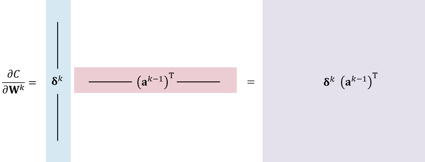
이렇게 각 행렬을 구해서 다 더하는 과정은 두 행렬곱을 열과 행의 외적의 합(Sum of Outer Products)[주재걸],[ML_Wiki]으로 보면 행렬과 행렬의 곱으로 이해할 수 있다. 즉 $\boldsymbol{\delta}^k_j$를 열로 가지는 행렬을 앞에 두고 $\mathbf{a}^{k-1}_j$를 행으로 가지는 행렬을 뒤에 두고 곱하면 같은 결과가 된다. 다음 그림이 이 과정을 설명하고 있다.

따라서 $\mathbf{W}^k$를 (out, in)인 행렬이라면 $\boldsymbol{\delta}^k$를 (out, m)행렬로 두고, $\mathbf{a}^{k-1}$를 (in,m)인 행렬로 두고 $\mathbf{a}^{k-1}$를 전치시켜 둘을 곱하면 크기가 (out,in)인 $\dfrac{\partial C}{\partial \mathbf{W}^k}$가 바로 구해진다.
한 걸음 더...
본 문서의 내용을 완전히 이해했다면 CNN의 역전파를 공부할 준비가 된 것이다. 다음 두 문서를 참고하여 CNN의 역전파 수식을 완전히 이해해보자.
CNN 역전파를 이해하는 가장 쉬운 방법The easiest way to understand CNN backpropagation https://metamath1.github.io/2017/01/23/CNN-backpropagation.html
합성곱 신경망에서 컨벌루션과 트랜스포즈드 컨벌루션의 관계 Relationship between Convolution and Transposed Convolution in CNN https://metamath1.github.io/2019/05/09/transconv.html
참고문헌
[cs231n] Backpropagation, Intuitions, http://cs231n.github.io/optimization-2/
[Ng] Backpropagation Intuition (C1W3L10), Andrew Ng, https://youtu.be/yXcQ4B-YSjQ
[임성빈] Matrix calculus, 임성빈, https://www.slideshare.net/ssuser7e10e4/matrix-calculus
[조준우] 벡터, 행렬에 대한 미분Derivatives for vectors and matrices, 조준우, https://metamath1.github.io/2018/01/02/matrix-derivatives.html
[Johnson] Derivatives, Backpropagation, and Vectorization, Justin Johnson, http://cs231n.stanford.edu/handouts/derivatives.pdf
[Goodfellow et. al] Deeplearning, MIT Press, 2016
[주재걸] 인공지능을 위한 선형대수, 주재걸, https://www.edwith.org/linearalgebra4ai
[ML_Wiki] Matrix-Matrix Multiplication, Matrix-Matrix Multiplication
%%html
<link href='https://fonts.googleapis.com/earlyaccess/notosanskr.css' rel='stylesheet' type='text/css'>
<!--https://github.com/kattergil/NotoSerifKR-Web/stargazers-->
<link href='https://cdn.rawgit.com/kattergil/NotoSerifKR-Web/5e08423b/stylesheet/NotoSerif-Web.css' rel='stylesheet' type='text/css'>
<!--https://github.com/Joungkyun/font-d2coding-->
<link href="http://cdn.jsdelivr.net/gh/joungkyun/font-d2coding/d2coding.css" rel="stylesheet" type="text/css">
<style>
    h1 { font-family: 'Noto Sans KR' !important; color:#348ABD !important;   }
    h2 { font-family: 'Noto Sans KR' !important; color:#467821 !important;   }
    h3 { font-family: 'Noto Sans KR' !important; color:#A60628 !important;   }
    h4 { font-family: 'Noto Sans KR' !important; color:#7A68A6 !important;   }

    p:not(.navbar-text) { font-family: 'Noto Serif KR', 'Nanum Myeongjo'; font-size: 11pt; line-height: 200%;  text-indent: 10px; }
    li:not(.dropdown):not(.p-TabBar-tab):not(.p-MenuBar-item):not(.jp-DirListing-item):not(.p-CommandPalette-header):not(.p-CommandPalette-item):not(.jp-RunningSessions-item):not(.p-Menu-item)
            { font-family: 'Noto Serif KR', 'Nanum Myeongjo'; font-size: 12pt; line-height: 200%; }
    table  { font-family: 'Noto Sans KR' !important;  font-size: 11pt !important; }
    li > p  { text-indent: 0px; }
    li > ul { margin-top: 0px !important; }
    sup { font-family: 'Noto Sans KR'; font-size: 9pt; }
    code, pre  { font-family: D2Coding, 'D2 coding' !important; font-size: 11pt !important; line-height: 130% !important;}
    .code-body { font-family: D2Coding, 'D2 coding' !important; font-size: 11pt !important;}
    .ns        { font-family: 'Noto Sans KR'; font-size: 15pt;}
    .summary   {
                   font-family: 'Georgia'; font-size: 12pt; line-height: 200%;
                   border-left:3px solid #D55E00;
                   padding-left:20px;
                   margin-top:10px;
                   margin-left:15px;
               }
    .green { color:#467821 !important; }
    .comment { font-family: 'Noto Sans KR'; font-size: 10pt; }
</style>