Tools
By convention, the first lines of code are always about importing the packages we'll use.
import pandas as pd
import numpy as np
import networkx as nx
Tutorials on pandas can be found at:
- https://pandas.pydata.org/pandas-docs/stable/10min.html
- https://pandas.pydata.org/pandas-docs/stable/tutorials.html
Tutorials on numpy can be found at:
- https://docs.scipy.org/doc/numpy/user/quickstart.html
- http://www.scipy-lectures.org/intro/numpy/index.html
- http://www.scipy-lectures.org/advanced/advanced_numpy/index.html
A tutorial on networkx can be found at:
Import the data
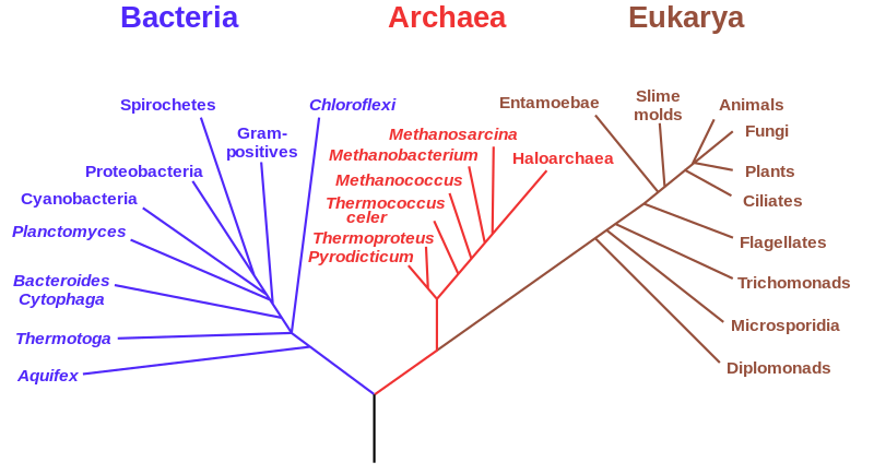
We will play with a excerpt of the Tree of Life, that can be found together with this notebook. This dataset is reduced to the first 1000 taxons (starting from the root node). The full version is available here: Open Tree of Life.
tree_of_life = pd.read_csv('data/taxonomy_small.tsv', sep='\t\|\t?', encoding='utf-8', engine='python')
If you do not remember the details of a function:
pd.read_csv?
For more info on the separator, see regex.
Now, what is the object tree_of_life? It is a Pandas DataFrame.
tree_of_life
| uid | parent_uid | name | rank | sourceinfo | uniqname | flags | Unnamed: 7 | |
|---|---|---|---|---|---|---|---|---|
| 0 | 805080 | NaN | life | no rank | silva:0,ncbi:1,worms:1,gbif:0,irmng:0 | NaN | NaN | NaN |
| 1 | 93302 | 805080.0 | cellular organisms | no rank | ncbi:131567 | NaN | NaN | NaN |
| 2 | 996421 | 93302.0 | Archaea | domain | silva:D37982/#1,ncbi:2157,worms:8,gbif:2,irmng:12 | Archaea (domain silva:D37982/#1) | NaN | NaN |
| 3 | 5246114 | 996421.0 | Marine Hydrothermal Vent Group 1(MHVG-1) | no rank - terminal | silva:AB302039/#2 | NaN | NaN | NaN |
| 4 | 102415 | 996421.0 | Thaumarchaeota | phylum | silva:D87348/#2,ncbi:651137,worms:559429,irmng... | NaN | NaN | NaN |
| ... | ... | ... | ... | ... | ... | ... | ... | ... |
| 994 | 5571591 | 102415.0 | uncultured marine thaumarchaeote KM3_175_A05 | species | ncbi:1456051 | NaN | environmental,not_otu | NaN |
| 995 | 5571756 | 102415.0 | uncultured marine thaumarchaeote KM3_46_E07 | species | ncbi:1456159 | NaN | environmental,not_otu | NaN |
| 996 | 5571888 | 102415.0 | uncultured marine thaumarchaeote KM3_02_A10 | species | ncbi:1455955 | NaN | environmental,not_otu | NaN |
| 997 | 5205131 | 102415.0 | thaumarchaeote enrichment culture clone Ec.FBa... | species | ncbi:1238015 | NaN | environmental | NaN |
| 998 | 5572032 | 102415.0 | uncultured marine thaumarchaeote KM3_53_B02 | species | ncbi:1456180 | NaN | environmental,not_otu | NaN |
999 rows × 8 columns
The description of the entries is given here: https://github.com/OpenTreeOfLife/reference-taxonomy/wiki/Interim-taxonomy-file-format
Explore the table
tree_of_life.columns
Index(['uid', 'parent_uid', 'name', 'rank', 'sourceinfo', 'uniqname', 'flags',
       'Unnamed: 7'],
      dtype='object')
Let us drop some columns.
tree_of_life = tree_of_life.drop(columns=['sourceinfo', 'uniqname', 'flags','Unnamed: 7'])
tree_of_life.head()
| uid | parent_uid | name | rank | |
|---|---|---|---|---|
| 0 | 805080 | NaN | life | no rank |
| 1 | 93302 | 805080.0 | cellular organisms | no rank |
| 2 | 996421 | 93302.0 | Archaea | domain |
| 3 | 5246114 | 996421.0 | Marine Hydrothermal Vent Group 1(MHVG-1) | no rank - terminal |
| 4 | 102415 | 996421.0 | Thaumarchaeota | phylum |
Pandas infered the type of values inside each column (int, float, string and string). The parent_uid column has float values because there was a missing value, converted to NaN
print(tree_of_life['uid'].dtype, tree_of_life.parent_uid.dtype)
int64 float64
How to access individual values.
tree_of_life.iloc[0, 2]
'life'
tree_of_life.loc[0, 'name']
'life'
Exercise: Guess the output of the following line:
# tree_of_life.uid[0] == tree_of_life.parent_uid[1]
Ordering the data.
tree_of_life.sort_values(by='name').head()
| uid | parent_uid | name | rank | |
|---|---|---|---|---|
| 297 | 5246638 | 102415.0 | AB64A-17 | no rank - terminal |
| 293 | 5246632 | 102415.0 | AK31 | no rank - terminal |
| 298 | 5246637 | 102415.0 | AK56 | no rank - terminal |
| 202 | 5246635 | 102415.0 | AK59 | no rank - terminal |
| 204 | 5246636 | 102415.0 | AK8 | no rank - terminal |
Remark: Some functions do not change the dataframe (option inline=False by default).
tree_of_life.head()
| uid | parent_uid | name | rank | |
|---|---|---|---|---|
| 0 | 805080 | NaN | life | no rank |
| 1 | 93302 | 805080.0 | cellular organisms | no rank |
| 2 | 996421 | 93302.0 | Archaea | domain |
| 3 | 5246114 | 996421.0 | Marine Hydrothermal Vent Group 1(MHVG-1) | no rank - terminal |
| 4 | 102415 | 996421.0 | Thaumarchaeota | phylum |
Operation on the columns
Unique values, useful for categories:
tree_of_life['rank'].unique()
array(['no rank', 'domain', 'no rank - terminal', 'phylum', 'species',
       'order', 'family', 'genus', 'class'], dtype=object)
Selecting only one category.
tree_of_life[tree_of_life['rank'] == 'species'].head()
| uid | parent_uid | name | rank | |
|---|---|---|---|---|
| 7 | 5205649 | 4795965.0 | uncultured marine crenarchaeote 'Gulf of Maine' | species |
| 8 | 5208050 | 4795965.0 | uncultured marine archaeon DCM858 | species |
| 9 | 5205092 | 4795965.0 | uncultured marine group I thaumarchaeote | species |
| 10 | 5205072 | 4795965.0 | uncultured Nitrosopumilaceae archaeon | species |
| 11 | 5208765 | 4795965.0 | uncultured marine archaeon DCM874 | species |
How many species do we have?
len(tree_of_life[tree_of_life['rank'] == 'species'])
912
tree_of_life['rank'].value_counts()
species               912
no rank - terminal     58
no rank                12
genus                   8
order                   3
family                  3
domain                  1
phylum                  1
class                   1
Name: rank, dtype: int64
Exercise: Display the entry with name 'Archaea', then display the entry of its parent.
# Your code here.
Building the graph
Let us build the adjacency matrix of the graph. For that we need to reorganize the data. First we separate the nodes and their properties from the edges.
nodes = tree_of_life[['uid', 'name','rank']]
edges = tree_of_life[['uid', 'parent_uid']]
When using an adjacency matrix, nodes are indexed by their row or column number and not by a uid. Let us create a new index for the nodes.
# Create a column for node index.
nodes.reset_index(level=0, inplace=True)
nodes = nodes.rename(columns={'index':'node_idx'})
nodes.head()
| node_idx | uid | name | rank | |
|---|---|---|---|---|
| 0 | 0 | 805080 | life | no rank |
| 1 | 1 | 93302 | cellular organisms | no rank |
| 2 | 2 | 996421 | Archaea | domain |
| 3 | 3 | 5246114 | Marine Hydrothermal Vent Group 1(MHVG-1) | no rank - terminal |
| 4 | 4 | 102415 | Thaumarchaeota | phylum |
# Create a conversion table from uid to node index.
uid2idx = nodes[['node_idx', 'uid']]
uid2idx = uid2idx.set_index('uid')
uid2idx.head()
| node_idx | |
|---|---|
| uid | |
| 805080 | 0 |
| 93302 | 1 |
| 996421 | 2 |
| 5246114 | 3 |
| 102415 | 4 |
edges.head()
| uid | parent_uid | |
|---|---|---|
| 0 | 805080 | NaN |
| 1 | 93302 | 805080.0 |
| 2 | 996421 | 93302.0 |
| 3 | 5246114 | 996421.0 |
| 4 | 102415 | 996421.0 |
Now we are ready to use yet another powerful function of Pandas. Those familiar with SQL will recognize it: the join function.
# Add a new column, matching the uid with the node_idx.
edges = edges.join(uid2idx, on='uid')
# Do the same with the parent_uid.
edges = edges.join(uid2idx, on='parent_uid', rsuffix='_parent')
# Drop the uids.
edges_renumbered = edges.drop(columns=['uid','parent_uid'])
The edges_renumbered table is a list of renumbered edges connecting each node to its parent.
edges_renumbered.head()
| node_idx | node_idx_parent | |
|---|---|---|
| 0 | 0 | NaN |
| 1 | 1 | 0.0 |
| 2 | 2 | 1.0 |
| 3 | 3 | 2.0 |
| 4 | 4 | 2.0 |
Building the (weighted) adjacency matrix
We will use numpy to build this matrix. Note that we don't have edge weights here, so our graph is going to be unweighted.
n_nodes = len(nodes)
adjacency = np.zeros((n_nodes, n_nodes), dtype=int)
for idx, row in edges.iterrows():
    if np.isnan(row.node_idx_parent):
        continue
    i, j = int(row.node_idx), int(row.node_idx_parent)
    adjacency[i, j] = 1  # weight
    adjacency[j, i] = 1  # weight to obtain an undirected network
adjacency[:15, :15]
array([[0, 1, 0, 0, 0, 0, 0, 0, 0, 0, 0, 0, 0, 0, 0],
       [1, 0, 1, 0, 0, 0, 0, 0, 0, 0, 0, 0, 0, 0, 0],
       [0, 1, 0, 1, 1, 0, 0, 0, 0, 0, 0, 0, 0, 0, 0],
       [0, 0, 1, 0, 0, 0, 0, 0, 0, 0, 0, 0, 0, 0, 0],
       [0, 0, 1, 0, 0, 1, 1, 0, 0, 0, 0, 0, 0, 0, 0],
       [0, 0, 0, 0, 1, 0, 0, 0, 0, 0, 0, 0, 0, 0, 0],
       [0, 0, 0, 0, 1, 0, 0, 1, 1, 1, 1, 1, 1, 0, 0],
       [0, 0, 0, 0, 0, 0, 1, 0, 0, 0, 0, 0, 0, 0, 0],
       [0, 0, 0, 0, 0, 0, 1, 0, 0, 0, 0, 0, 0, 0, 0],
       [0, 0, 0, 0, 0, 0, 1, 0, 0, 0, 0, 0, 0, 0, 0],
       [0, 0, 0, 0, 0, 0, 1, 0, 0, 0, 0, 0, 0, 0, 0],
       [0, 0, 0, 0, 0, 0, 1, 0, 0, 0, 0, 0, 0, 0, 0],
       [0, 0, 0, 0, 0, 0, 1, 0, 0, 0, 0, 0, 0, 1, 0],
       [0, 0, 0, 0, 0, 0, 0, 0, 0, 0, 0, 0, 1, 0, 1],
       [0, 0, 0, 0, 0, 0, 0, 0, 0, 0, 0, 0, 0, 1, 0]])
Congratulations, you have built the adjacency matrix!
The graph
# A simple command to create the graph from the adjacency matrix.
graph = nx.from_numpy_array(adjacency)
In addition, let us add some attributes to the nodes:
node_props = nodes.to_dict()
for key in node_props:
    # print(key, node_props[key])
    nx.set_node_attributes(graph, node_props[key], key)
Let us check if it is correctly recorded:
graph.node[1]
{'node_idx': 1, 'uid': 93302, 'name': 'cellular organisms', 'rank': 'no rank'}
Exercise 1:
Build the graph directly from the edges table (without using the adjacency matrix).
# Your code here.
Exercise 2:
Build the graph from the initial tree_of_life table by directly iterating over the rows of this table (without building the adjacency matrix).
# Your code here.
Exercise 3:
Get the adjacency matrix with nx.adjacency_matrix(graph) and compare it with what we obtained previously.
# Your code here.
Graph visualization
To conclude, let us visualize the graph. We will use the python module networkx.
The following line is a magic command. It enables plotting inside the notebook.
%matplotlib inline
You may also try %matplotlib notebook for a zoomable version of plots.
Draw the graph with two different layout algorithms.
nx.draw_spectral(graph)
/home/michael/.conda/envs/ntds_2019/lib/python3.7/site-packages/networkx/drawing/nx_pylab.py:579: MatplotlibDeprecationWarning:
The iterable function was deprecated in Matplotlib 3.1 and will be removed in 3.3. Use np.iterable instead.
  if not cb.iterable(width):

nx.draw_spring(graph)

Save the graph to disk in the gexf format, readable by gephi and other tools that manipulate graphs. You may now explore the graph using gephi and compare the visualizations.
nx.write_gexf(graph, 'tree_of_life.gexf')