Google Images Classifier with fastai
%reload_ext autoreload
%autoreload 2
%matplotlib inline
import os
import numpy as np
import pandas as pd
from glob import glob
from pathlib import Path
from collections import Counter
import torch
from tqdm.auto import tqdm
from tqdm import tqdm_notebook
tqdm.pandas()
from fastai.basic_data import DatasetType
from fastai.metrics import error_rate, accuracy
from fastai.vision import models as vision_models
from fastai.vision import download_images, verify_images
from fastai.vision import ClassificationInterpretation, ImageDataBunch, imagenet_stats, cnn_learner
from fastai.widgets import ImageCleaner, DatasetFormatter
NUM_CORES = 4
CSV_DATA_PATH = Path(os.path.join('data', 'casino'))
IMAGE_DATA_PATH = CSV_DATA_PATH/'images'
Get a list of URLs
Search and scroll
Go to Google Images and search for the images you are interested in. The more specific you are in your Google Search, the better the results and the less manual pruning you will have to do.
Scroll down until you've seen all the images you want to download, or until you see a button that says 'Show more results'. All the images you scrolled past are now available to download. To get more, click on the button, and continue scrolling. The maximum number of images Google Images shows is 700.
It is a good idea to put things you want to exclude into the search query, for instance if you are searching for the Eurasian wolf, "canis lupus lupus", it might be a good idea to exclude other variants:
"canis lupus lupus" -dog -arctos -familiaris -baileyi -occidentalis
You can also limit your results to show only photos by clicking on Tools and selecting Photos from the Type dropdown.
Download into file
Now you must run some Javascript code in your browser which will save the URLs of all the images you want for you dataset.
Press CtrlShiftJ in Windows/Linux and CmdOptJ in Mac, and a small window the javascript 'Console' will appear. That is where you will paste the JavaScript commands.
You will need to get the urls of each of the images. Before running the following commands, you may want to disable ad blocking extensions (uBlock, AdBlockPlus etc.) in Chrome. Otherwise the window.open() command doesn't work. Then you can run the following commands:
urls = Array.from(document.querySelectorAll('.rg_di .rg_meta')).map(el=>JSON.parse(el.textContent).ou);
window.open('data:text/csv;charset=utf-8,' + escape(urls.join('\n')));
# https://docs.fast.ai/vision.data.html#Building-your-own-dataset
classes = ['craps', 'roulette', 'blackjack']
for class_ in classes:
data_path = IMAGE_DATA_PATH/class_
data_path.mkdir(parents=True, exist_ok=True)
download_images(CSV_DATA_PATH/class_, data_path, max_pics=256)
classes = ['craps', 'roulette', 'blackjack']
for class_ in classes:
data_path = IMAGE_DATA_PATH/class_
verify_images(data_path, delete=True, max_size=512)
Create Dataset
classes = ['craps', 'roulette', 'blackjack']
dataset = ImageDataBunch.from_folder(IMAGE_DATA_PATH, train='.', valid_pct=0.2, seed=21, size=224, num_workers=4).normalize(imagenet_stats)
dataset
ImageDataBunch; Train: LabelList (541 items) x: ImageList Image (3, 224, 224),Image (3, 224, 224),Image (3, 224, 224),Image (3, 224, 224),Image (3, 224, 224) y: CategoryList craps,craps,craps,craps,craps Path: data/casino/images; Valid: LabelList (135 items) x: ImageList Image (3, 224, 224),Image (3, 224, 224),Image (3, 224, 224),Image (3, 224, 224),Image (3, 224, 224) y: CategoryList blackjack,blackjack,craps,blackjack,roulette Path: data/casino/images; Test: None
dataset.classes
['blackjack', 'craps', 'roulette']
dataset.show_batch(rows=3, fig_size=(3, 3))

dataset.c
3
Training Model
learn = cnn_learner(dataset, vision_models.resnet34, metrics=[error_rate])
learn.fit_one_cycle(4)
| epoch | train_loss | valid_loss | error_rate | time |
|---|---|---|---|---|
| 0 | 1.494553 | 0.273171 | 0.088889 | 00:08 |
| 1 | 0.857744 | 0.273497 | 0.074074 | 00:05 |
| 2 | 0.584896 | 0.255926 | 0.081481 | 00:05 |
| 3 | 0.449855 | 0.252822 | 0.088889 | 00:05 |
learn.recorder.plot_losses()

learn.save('resnet34', return_path=True)
PosixPath('data/casino/images/models/resnet34.pth')
Optimizing Learning rate
# If the plot is not showing try to give a start and end learning rate
# learn.lr_find(start_lr=1e-5, end_lr=1e-1)
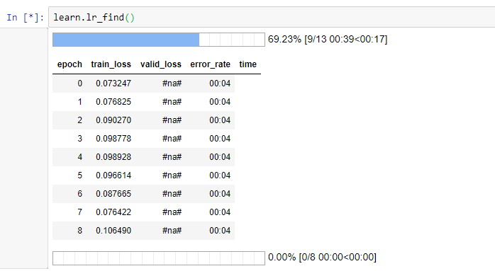
learn.lr_find()
LR Finder is complete, type {learner_name}.recorder.plot() to see the graph.
learn.recorder.plot(suggestion=True)
Min numerical gradient: 6.31E-07 Min loss divided by 10: 7.59E-08

print("From: {:.20f}".format(6.31E-07), "To: {:.20f}".format(3e-4))
From: 0.00000063100000000000 To: 0.00029999999999999997
learn.unfreeze()
learn.fit_one_cycle(4, max_lr=slice(1.10E-06, 3e-4))
| epoch | train_loss | valid_loss | error_rate | time |
|---|---|---|---|---|
| 0 | 0.095168 | 0.236067 | 0.074074 | 00:07 |
| 1 | 0.073059 | 0.209149 | 0.074074 | 00:07 |
| 2 | 0.060378 | 0.203401 | 0.059259 | 00:07 |
| 3 | 0.053346 | 0.204234 | 0.059259 | 00:07 |
learn.recorder.plot_losses()

learn.save('resnet34', return_path=True)
PosixPath('data/casino/images/models/resnet34.pth')
Interpretation
learn = cnn_learner(dataset, vision_models.resnet34, metrics=[error_rate])
learn.load('resnet34');
cls_interpreter = ClassificationInterpretation.from_learner(learn)
cls_interpreter.plot_top_losses(k=9, figsize=(12, 12))

cls_interpreter.plot_confusion_matrix(figsize=(6,6), dpi=60)

cls_interpreter.most_confused(min_val=1)
[('craps', 'blackjack', 3),
('blackjack', 'craps', 2),
('blackjack', 'roulette', 2),
('roulette', 'craps', 1)]
Doing the cleanup using DataFormatter Widget
# Loading model with ImageDataBunch containing all images (i.e. without validation split)
dataset_all = ImageDataBunch.from_folder(IMAGE_DATA_PATH, train='.', valid_pct=0.0, size=224).normalize(imagenet_stats)
dataset_all
ImageDataBunch; Train: LabelList (676 items) x: ImageList Image (3, 224, 224),Image (3, 224, 224),Image (3, 224, 224),Image (3, 224, 224),Image (3, 224, 224) y: CategoryList craps,craps,craps,craps,craps Path: data/casino/images; Valid: LabelList (0 items) x: ImageList y: CategoryList Path: data/casino/images; Test: None
learn = cnn_learner(dataset_all, vision_models.resnet34, metrics=[error_rate])
learn.load('resnet34');
ds, indexes = DatasetFormatter.from_toplosses(learn)
ds
LabelList (676 items) x: ImageList Image (3, 250, 300),Image (3, 250, 300),Image (3, 250, 300),Image (3, 250, 300),Image (3, 250, 300) y: CategoryList craps,craps,craps,craps,craps Path: data/casino/images
ImageCleaner(ds, indexes, CSV_DATA_PATH)
HBox(children=(VBox(children=(Image(value=b'\xff\xd8\xff\xe0\x00\x10JFIF\x00\x01\x01\x01\x00d\x00d\x00\x00\xff…
Button(button_style='primary', description='Next Batch', layout=Layout(width='auto'), style=ButtonStyle())
ds, indexes = DatasetFormatter().from_similars(learn)
ds
Getting activations...
Computing similarities...
LabelList (676 items) x: ImageList Image (3, 250, 300),Image (3, 250, 300),Image (3, 250, 300),Image (3, 250, 300),Image (3, 250, 300) y: CategoryList craps,craps,craps,craps,craps Path: data/casino/images
ImageCleaner(ds, indexes, CSV_DATA_PATH, duplicates=True)
HBox(children=(VBox(children=(Image(value=b'\xff\xd8\xff\xe0\x00\x10JFIF\x00\x01\x01\x01\x00d\x00d\x00\x00\xff…
Button(button_style='primary', description='Next Batch', layout=Layout(width='auto'), style=ButtonStyle())
Re-Building Model after Cleanup
dataset_cleaned = ImageDataBunch.from_csv(CSV_DATA_PATH, folder='.', csv_labels='cleaned.csv', valid_pct=0.2, size=224).normalize(imagenet_stats)
dataset_cleaned
ImageDataBunch; Train: LabelList (520 items) x: ImageList Image (3, 224, 224),Image (3, 224, 224),Image (3, 224, 224),Image (3, 224, 224),Image (3, 224, 224) y: CategoryList craps,craps,craps,craps,craps Path: data/casino; Valid: LabelList (129 items) x: ImageList Image (3, 224, 224),Image (3, 224, 224),Image (3, 224, 224),Image (3, 224, 224),Image (3, 224, 224) y: CategoryList craps,craps,roulette,roulette,craps Path: data/casino; Test: None
dataset.classes
['blackjack', 'craps', 'roulette']
learn = cnn_learner(dataset, vision_models.resnet34, metrics=[error_rate])
learn.fit_one_cycle(6)
| epoch | train_loss | valid_loss | error_rate | time |
|---|---|---|---|---|
| 0 | 1.690365 | 0.552709 | 0.177778 | 00:05 |
| 1 | 1.027674 | 0.332303 | 0.096296 | 00:05 |
| 2 | 0.717548 | 0.288599 | 0.059259 | 00:05 |
| 3 | 0.526696 | 0.292895 | 0.059259 | 00:05 |
| 4 | 0.410802 | 0.278058 | 0.059259 | 00:05 |
| 5 | 0.324657 | 0.274076 | 0.059259 | 00:05 |
learn.recorder.plot_losses()

learn.save('resnet34', return_path=True)
PosixPath('data/casino/images/models/resnet34.pth')
learn.lr_find(start_lr=1e-5, end_lr=1e-1)
LR Finder is complete, type {learner_name}.recorder.plot() to see the graph.
learn.recorder.plot(suggestion=True)
Min numerical gradient: 3.31E-05 Min loss divided by 10: 7.59E-04

learn.unfreeze()
learn.fit_one_cycle(4, max_lr=slice(3.31E-05, 3e-4))
| epoch | train_loss | valid_loss | error_rate | time |
|---|---|---|---|---|
| 0 | 0.089379 | 0.286874 | 0.059259 | 00:07 |
| 1 | 0.079444 | 0.358506 | 0.081481 | 00:07 |
| 2 | 0.068128 | 0.300093 | 0.044444 | 00:07 |
| 3 | 0.057651 | 0.277920 | 0.051852 | 00:07 |
learn.recorder.plot_losses()

learn.save('resnet34', return_path=True)
PosixPath('data/casino/images/models/resnet34.pth')
cls_interpreter = ClassificationInterpretation.from_learner(learn)
cls_interpreter.plot_top_losses(k=9, figsize=(12, 12))

cls_interpreter.plot_confusion_matrix(figsize=(6,6), dpi=60)

Model in production
learn.export('resnet34_prod.pkl')
Deployment API code can be found in lesson2_production.py
Things that can go wrong
- Most of the time things will train fine with the defaults
- There's not much you really need to tune (despite what you've heard!)
- Most likely are
- Learning rate
- Number of epochs
Learning rate (LR) too high
learn = cnn_learner(dataset, vision_models.resnet34, metrics=error_rate)
learn.fit_one_cycle(1, max_lr=0.5)
| epoch | train_loss | valid_loss | error_rate | time |
|---|---|---|---|---|
| 0 | 21.222269 | 325215360.000000 | 0.644444 | 00:22 |
When the validation loss go through the roof your learning rate is too high IMO!
Learning rate (LR) too low
As well as taking a really long time, it's getting too many looks at each image, so may overfit.
learn = cnn_learner(dataset, vision_models.resnet34, metrics=error_rate)
learn.fit_one_cycle(10, max_lr=1e-5)
| epoch | train_loss | valid_loss | error_rate | time |
|---|---|---|---|---|
| 0 | 1.879741 | 1.873090 | 0.711111 | 00:06 |
| 1 | 1.807466 | 1.545421 | 0.688889 | 00:05 |
| 2 | 1.841128 | 1.434029 | 0.651852 | 00:06 |
| 3 | 1.800319 | 1.358002 | 0.592593 | 00:06 |
| 4 | 1.765320 | 1.304487 | 0.562963 | 00:05 |
| 5 | 1.754511 | 1.267466 | 0.562963 | 00:05 |
| 6 | 1.724406 | 1.245595 | 0.555556 | 00:06 |
| 7 | 1.713679 | 1.232486 | 0.548148 | 00:06 |
| 8 | 1.687130 | 1.226034 | 0.540741 | 00:06 |
| 9 | 1.675795 | 1.227245 | 0.555556 | 00:06 |
learn.recorder.plot_metrics()

When the validation loss is decreasing very slowly zzzzzzzzzzzzzzzzzzzzzzzzzzzzzzzzz your learning rate is too low IMO!
Too few epochs
learn = cnn_learner(dataset, vision_models.resnet34, metrics=error_rate)
learn.fit_one_cycle(1)
| epoch | train_loss | valid_loss | error_rate | time |
|---|---|---|---|---|
| 0 | 1.107221 | 0.346638 | 0.103704 | 00:06 |
Large difference between train_loss and valid_loss and you have too few epochs IMO!
Too many epochs
learn = cnn_learner(dataset, vision_models.resnet34, metrics=error_rate)
learn.unfreeze()
learn.fit_one_cycle(40)
| epoch | train_loss | valid_loss | error_rate | time |
|---|---|---|---|---|
| 0 | 1.282991 | 0.726441 | 0.355556 | 00:07 |
| 1 | 0.945720 | 0.327931 | 0.133333 | 00:07 |
| 2 | 0.685992 | 0.234257 | 0.081481 | 00:07 |
| 3 | 0.499212 | 0.183728 | 0.066667 | 00:07 |
| 4 | 0.377004 | 0.170877 | 0.037037 | 00:07 |
| 5 | 0.294681 | 0.187047 | 0.037037 | 00:07 |
| 6 | 0.232047 | 0.212903 | 0.029630 | 00:07 |
| 7 | 0.189293 | 0.239343 | 0.051852 | 00:07 |
| 8 | 0.155400 | 0.242453 | 0.051852 | 00:07 |
| 9 | 0.132623 | 0.218016 | 0.044444 | 00:07 |
| 10 | 0.115849 | 0.206627 | 0.044444 | 00:07 |
| 11 | 0.100240 | 0.212578 | 0.059259 | 00:07 |
| 12 | 0.084683 | 0.261154 | 0.059259 | 00:07 |
| 13 | 0.071741 | 0.214044 | 0.059259 | 00:07 |
| 14 | 0.064226 | 0.209822 | 0.037037 | 00:07 |
| 15 | 0.057190 | 0.193891 | 0.051852 | 00:07 |
| 16 | 0.053428 | 0.166092 | 0.059259 | 00:07 |
| 17 | 0.049568 | 0.138359 | 0.051852 | 00:07 |
| 18 | 0.043058 | 0.150081 | 0.051852 | 00:07 |
| 19 | 0.044299 | 0.167534 | 0.051852 | 00:07 |
| 20 | 0.044031 | 0.432090 | 0.096296 | 00:07 |
| 21 | 0.046774 | 0.402418 | 0.111111 | 00:07 |
| 22 | 0.051132 | 0.476849 | 0.096296 | 00:07 |
| 23 | 0.057292 | 0.457212 | 0.081481 | 00:07 |
| 24 | 0.055693 | 0.325403 | 0.074074 | 00:07 |
| 25 | 0.057003 | 0.226553 | 0.051852 | 00:07 |
| 26 | 0.054376 | 0.232475 | 0.051852 | 00:07 |
| 27 | 0.048215 | 0.189798 | 0.037037 | 00:07 |
| 28 | 0.044361 | 0.191182 | 0.037037 | 00:07 |
| 29 | 0.039331 | 0.209269 | 0.044444 | 00:07 |
| 30 | 0.035801 | 0.181996 | 0.051852 | 00:07 |
| 31 | 0.032069 | 0.155043 | 0.037037 | 00:07 |
| 32 | 0.027474 | 0.146985 | 0.029630 | 00:07 |
| 33 | 0.024649 | 0.144802 | 0.029630 | 00:07 |
| 34 | 0.021711 | 0.143405 | 0.022222 | 00:07 |
| 35 | 0.018487 | 0.143665 | 0.022222 | 00:07 |
| 36 | 0.015770 | 0.142340 | 0.022222 | 00:07 |
| 37 | 0.014120 | 0.142183 | 0.022222 | 00:07 |
| 38 | 0.012971 | 0.141440 | 0.022222 | 00:07 |
| 39 | 0.011653 | 0.141028 | 0.022222 | 00:07 |
When your error_rate start increasing after decrease you are overfitting IMO!
Stochastic Gradient Descent a.k.a. Computer's do Gradient Descent :P
%matplotlib inline
from fastai.basics import torch, nn, plt, mse, tensor, np
Linear regression problem
y = mx + c
tecnically, m = gradient of line (a.k.a. slope of line), c = intercept of line (rank 1 tensor), x = rank 2 tensor (dependent variable)
n = 100
x = torch.ones(n, 2)
x.shape
torch.Size([100, 2])
x[:5]
tensor([[1., 1.],
[1., 1.],
[1., 1.],
[1., 1.],
[1., 1.]])
x[:, 0].uniform_(-1.,1)
x[:5]
tensor([[ 0.8115, 1.0000],
[-0.9355, 1.0000],
[-0.3264, 1.0000],
[-0.5824, 1.0000],
[ 0.9377, 1.0000]])
m = tensor(3., 2)
m
tensor([3., 2.])
y = x@m + torch.rand(n)
plt.scatter(x[:,0], y);

You want to find parameters (weights) m such that you minimize the error between the points and the line x@m. Note that here m is unknown. For a regression problem the most common error function or loss function is the mean squared error.
def mse(y_hat, y):
return ((y_hat-y)**2).mean()
Suppose we believe m = (-1.0,1.0) then we can compute y_hat which is our prediction and then compute our error.
m = tensor(-1., 1)
y_hat = x@m
mse(y_hat, y)
tensor(8.2945)
plt.scatter(x[:,0],y)
plt.scatter(x[:,0],y_hat);

So far we have specified the model (linear regression) and the evaluation criteria (or loss function). Now we need to handle optimization; that is, how do we find the best values for m? How do we find the best fitting linear regression.
Enter Gradient Descent
We would like to find the values of m that minimize mse_loss.
Gradient descent is an algorithm that minimizes functions. Given a function defined by a set of parameters, gradient descent starts with an initial set of parameter values and iteratively moves toward a set of parameter values that minimize the function. This iterative minimization is achieved by taking steps in the negative direction of the function gradient.
m = nn.Parameter(m)
m
Parameter containing: tensor([-1., 1.], requires_grad=True)
def update():
# calculate new y_hat
y_hat = x@m
# calculate loss a.k.a mean_squared_error
loss = mse(y, y_hat)
if t % 10 == 0: print(loss)
# calculate gradients w.r.t. loss a.k.a. mean_squared_error
loss.backward()
# do not include enclosed steps in gradient calculations
with torch.no_grad():
# subtract current slope value with its gradients multiplied by learning rate
# (i.e. do a certain fraction of update on gradients, the fraction is defined by learning rate)
m.sub_(lr * m.grad)
# zero the gradient values
m.grad.zero_()
1e-1
0.1
lr = 0.1 # take only 10% of gradient update into account
for t in range(100):
update()
tensor(8.2945, grad_fn=<MeanBackward0>) tensor(1.4955, grad_fn=<MeanBackward0>) tensor(0.5030, grad_fn=<MeanBackward0>) tensor(0.2110, grad_fn=<MeanBackward0>) tensor(0.1217, grad_fn=<MeanBackward0>) tensor(0.0943, grad_fn=<MeanBackward0>) tensor(0.0859, grad_fn=<MeanBackward0>) tensor(0.0834, grad_fn=<MeanBackward0>) tensor(0.0826, grad_fn=<MeanBackward0>) tensor(0.0823, grad_fn=<MeanBackward0>)
plt.scatter(x[:,0],y)
plt.scatter(x[:,0],x@m);

Animate it (code as is!)
from matplotlib import animation, rc
rc('animation', html='jshtml')
m = nn.Parameter(tensor(-1.,1))
fig = plt.figure()
plt.scatter(x[:,0], y, c='orange')
line, = plt.plot(x[:,0], x@m)
plt.close()
def animate(i):
update()
line.set_ydata(x@m)
return line,
animation.FuncAnimation(fig, animate, np.arange(0, 100), interval=20)
In practice, we don't calculate on the whole file at once, but we use mini-batches.
Vocab
- Learning rate
- Some defined fraction that will be multipled with the gradients before update.
- Epoch
- One complete run throught the dataset, i.e. one full run of computing and updating gradients after observing all records in training set.
- Minibatch
- Partial observations taken into considerations while calculating loss.
- SGD
- The gradient descent of computers.
- Model / Architecture
- A pre-defined equation of variables a.k.a. rank 2 tensors that do not change.
- Parameters
- The gradients that undergo update and are multiplied with variables.
- Loss function
- Something that calculates the basis for calculating gradients.
For classification problems, we use cross entropy loss, also known as negative log likelihood loss. This penalizes incorrect confident predictions, and correct unconfident predictions.