 ***
# Lecture 3 - Gradient Descent
***
$\newcommand{\vct}[1]{\mathbf{#1}}$
$\newcommand{\mtx}[1]{\mathbf{#1}}$
$\newcommand{\e}{\varepsilon}$
$\newcommand{\norm}[1]{\|#1\|}$
$\newcommand{\minimize}{\text{minimize}\quad}$
$\newcommand{\maximize}{\text{maximize}\quad}$
$\newcommand{\subjto}{\quad\text{subject to}\quad}$
$\newcommand{\R}{\mathbb{R}}$
$\newcommand{\trans}{T}$
$\newcommand{\ip}[2]{\langle {#1}, {#2} \rangle}$
$\newcommand{\zerovct}{\vct{0}}$
$\newcommand{\diff}[1]{\mathrm{d}{#1}}$
***
# Lecture 3 - Gradient Descent
***
$\newcommand{\vct}[1]{\mathbf{#1}}$
$\newcommand{\mtx}[1]{\mathbf{#1}}$
$\newcommand{\e}{\varepsilon}$
$\newcommand{\norm}[1]{\|#1\|}$
$\newcommand{\minimize}{\text{minimize}\quad}$
$\newcommand{\maximize}{\text{maximize}\quad}$
$\newcommand{\subjto}{\quad\text{subject to}\quad}$
$\newcommand{\R}{\mathbb{R}}$
$\newcommand{\trans}{T}$
$\newcommand{\ip}[2]{\langle {#1}, {#2} \rangle}$
$\newcommand{\zerovct}{\vct{0}}$
$\newcommand{\diff}[1]{\mathrm{d}{#1}}$
Most modern optimization methods are iterative: they generate a sequence of points $\vct{x}_0,\vct{x}_1,\dots$ in $\R^n$ in the hope that this sequences will converge to a local or global minimizer $\vct{x}^*$ of a function $f(\vct{x})$. A typical rule for generating such a sequence would be to start with a vector $\vct{x}_0$, chosen by an educated guess, and then for $k\geq 0$, move from step $k$ to $k+1$ by
\begin{equation*} \vct{x}_{k+1} = \vct{x}_k+\alpha_k\vct{p}_k, \end{equation*}in a way that ensures that $f(\vct{x}_{k+1})\leq f(\vct{x}_k)$. The parameter $\alpha_k$ is called the step length, while $\vct{p}_k$ is the search direction. In this lecture we discuss one such method, the method of gradient descent, or steepest descent, and discuss how to select the right step length.
In the method of gradient descent, the search direction is chosen as
\begin{equation*} \vct{p}_k = -\nabla f(\vct{x}_k). \end{equation*}To see why this makes sense, let $\vct{p}$ be a direction and consider the Taylor expansion
\begin{equation*} f(\vct{x}_k+\alpha \vct{p}) = f(\vct{x}_k)+\alpha \ip{\vct{p}}{\nabla f(\vct{x}_k)}+O(\alpha^2). \end{equation*}Considering this as a function of $\alpha$, the rate of change in direction $\vct{p}$ at $\vct{x}_k$ is the derivative of this function at $\alpha=0$,
\begin{equation*} \frac{\diff{f}(\vct{x}_k+\alpha \vct{p})}{\diff{\alpha}}|_{\alpha=0} = \ip{\vct{p}}{\nabla f(\vct{x}_k)}, \end{equation*}also known as the directional derivative of $f$ at $\vct{x}_k$ in the direction $\vct{p}$. This formula indicates that the rate of change is negative, and we have a descent direction, if $\ip{\vct{p}}{\nabla f(\vct{x}_k)}<0$.
The Cauchy-Schwarz inequality (see Preliminaries, Page 9) gives the bounds
\begin{equation*} -\norm{\vct{p}}_2 \norm{\nabla f(\vct{x}_k)}_2 \leq \ip{\vct{p}}{\nabla f(\vct{x}_k)} \leq \norm{\vct{p}}_2 \norm{\nabla f(\vct{x}_k)}_2. \end{equation*}We see that the rate of change is the smallest when the first inequality is an equality, which happens if
\begin{equation*} \vct{p} = -\alpha \nabla f(\vct{x}_k) \end{equation*}for some $\alpha>0$.
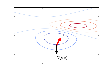
For a visual interpretation of what it means to be a descent direction, note that the angle $\theta$ between a vector $\vct{p}$ and the gradient $\nabla f(\vct{x})$ at a point $\vct{x}$ is given by (see Preliminaries, Page 9)
\begin{equation*} \ip{\vct{x}}{\nabla f(\vct{x})} = \norm{\vct{p}}_2\norm{\nabla f(\vct{x})}_2 \cos(\theta). \end{equation*}This is negative if the vector $\vct{p}$ forms and angle greater than $\pi/2$ with the gradient. Recall that the gradient points in the direction of steepest ascent, and is orthogonal to the level sets. If you are standing on the slope of a mountain, walking along the level set lines will not change your elevation, the gradient points to the steepest upward direction, and the negative gradient to the steepest descent.
Any multiple $\alpha \nabla f(\vct{x}_k)$ points in the direction of steepest descent, but we have to choose a sensible parameter $\alpha$ to ensure that we make sufficient progress, but at the same time don't overshoot. Ideally, we would choose the value $\alpha_k$ that minimizes $f(\vct{x}_k-\alpha_k \nabla f(\vct{x}_k))$. While finding such a minimizer is in general not easy, for quadratic functions in can be given in closed form.
Consider a function of the form
\begin{equation*} f(\vct{x}) = \frac{1}{2}\norm{\mtx{A}\vct{x}-\vct{b}}_2^2. \end{equation*}In Problem Sheet 1 you will show that that the Hessian is symmetric and positive semidefinite, with the gradient given by
\begin{equation*} \nabla f(\vct{x}) = \mtx{A}^{\trans}(\mtx{A}\vct{x}-\vct{b}). \end{equation*}The method of gradient descent proceeds as
\begin{equation*} \vct{x}_{k+1} = \vct{x}_k-\alpha_k \mtx{A}^{\top}(\mtx{A}\vct{x}_k-\vct{b}). \end{equation*}To find the best $\alpha_k$, we compute the minimum of the function
[1] \begin{equation*} \alpha \mapsto f(\vct{x}_k-\alpha \mtx{A}^{\trans}(\mtx{A}\vct{x}_k-\vct{b})). \end{equation*}
If we set $\vct{r}_k:=\mtx{A}^{\trans}(\vct{b}-\mtx{A}\vct{x}_k) = -\nabla f(\vct{x}_k)$ and compute the minimum of [1] by differentiating, we get the step length
\begin{equation*} \alpha_k = \frac{\vct{r}_k^{\trans}\vct{r}_k}{\vct{r}_k^{\trans}\mtx{A}^\trans\mtx{A}\vct{r}_k} = \frac{\norm{\vct{r}_k}_2^2}{\norm{\mtx{A}\vct{r}_k}_2^2}. \end{equation*}(Verify this!) Note also that when we have $\vct{r}_k$ and $\alpha_k$, we can compute the next $\vct{r}_k$ as
\begin{align*} r_{k+1} &= \mtx{A}^{\trans}(\vct{b}-\mtx{A}\vct{x}_{k+1})\\ &= \mtx{A}^{\trans}(\vct{b}-\mtx{A}(\vct{x}_{k}+\alpha_k \vct{r}_k))\\ &= \mtx{A}^{\trans}(\vct{b}-\mtx{A}\vct{x}_k - \alpha_k \mtx{A}^{\trans}\mtx{A}\vct{r}_k) = \vct{r}_k - \alpha_k \mtx{A}^{\trans}\mtx{A}\vct{r}_k. \end{align*}The gradient descent algorithm for the linear least squares problem proceeds by first computing $\vct{r}_0=\mtx{A}^{\trans}(\vct{b}-\mtx{A}\vct{x}_0)$, and then at each step
\begin{align*} \alpha_k &= \frac{\vct{r}_k^{\trans}\vct{r}_k}{\vct{r}_k^{\trans}\mtx{A}^\trans\mtx{A}\vct{r}_k}\\ \vct{x}_{k+1} &= \vct{x}_k+\alpha_k \vct{r}_k\\ \vct{r}_{k+1} &= \vct{r}_k - \alpha_{k}\mtx{A}^{\trans}\mtx{A}\vct{r}_k. \end{align*}Does this work? How do we know when to stop? It is worth noting that the residual satisfies $\vct{r}=0$ if and only if $\vct{x}$ is a stationary point, in our case, a minimizer. One criteria for stopping could then be to check whether $\norm{\vct{r}_k}_2\leq \e$ for some given tolerance $\e>0$. One potential problem with this criterion is that the function can become flat long before reaching a minimum, so an alternative stopping method would be to stop when the difference between two successive points, $\norm{\vct{x}_{k+1}-\vct{x}_k}_2$, becomes smaller than some $\e>0$.
Example. We plot the trajectory of gradient descent with the data \begin{equation*} \mtx{A} = \begin{pmatrix} 2 & 0\\ 1 & 3\\ 0 & 1 \end{pmatrix}, \quad \vct{b} = \begin{pmatrix} 1\\ -1\\ 0 \end{pmatrix}. \end{equation*}
The Python code below implements the gradient descent algorithm above. The stopping criteria used is that the residual $\vct{r}_k$ becomes smaller than the tolerance in the 2-norm.
import numpy as np
import numpy.linalg as la
import matplotlib.pyplot as plt

# The function graddesc performs the gradient descent algorithm with starting value x and tolerance tol
def graddesc(A, b, x, tol):
    """
    Input: matrix A, vector b, vector x, tolarance tol
    Output: trajectory of points x_0,x_1,... of the gradient descent method
    """
    # Compute the negative gradient r = A^T(b-Ax)
    r = np.dot(A.transpose(),b-np.dot(A,x))
    # Start with an empty array
    xout = [x]
    while la.norm(r,2) > tol:
        # If the gradient is bigger than the tolerance
        Ar = np.dot(A,r)
        alpha = np.dot(r,r)/np.dot(Ar,Ar)
        x = x + alpha*r
        xout.append(x)
        r = r-alpha*np.dot(A.transpose(),Ar)
    return np.array(xout).transpose()

# Define the matrix A and the vector b for the problem we consider, as well as the zero starting point
A = np.array([[2,0], [1,3], [0,1]])
b = np.array([1, -1, 0])
tol = 1e-4
x = np.zeros(2)

# Call the gradient descent function with input A and with starting value x=0
traj = graddesc(A, b, x, tol)

# Plot
%matplotlib inline

# Define the function we aim to minimize
def f(x):
    return np.dot(np.dot(A,x)-b,np.dot(A,x)-b)

# Determine the values of the function for the first 7 steps
# This is used to specify the location of the level sets
fvals = []
for i in range(7):
    fvals.append(f(traj[:,i]))

# Create a mesh grid for plotting the contours / level sets
xx = np.linspace(0.1,0.5,100)
yy = np.linspace(-0.5,-0.1,100)
X, Y = np.meshgrid(xx, yy)
Z = np.zeros(X.shape)
for i in range(Z.shape[0]):
    for j in range(Z.shape[1]):
        Z[i,j] = f(np.array([X[i,j], Y[i,j]]))

# Get a nice monotone colormap
cmap = plt.cm.get_cmap("coolwarm")

# Plot the contours and the trajectory
plt.contour(X, Y, Z, cmap = cmap, levels = list(reversed(fvals)))
plt.plot(traj[0,:], traj[1,:], 'o-k')
#plt.axis('off')
plt.xlim([0.1,0.5])
plt.ylim([-0.5,-0.15])
plt.axis('equal')
plt.show()
