(Very brief) Introduction to Python and Jupyter
Welcome! This introduction will get you started with Python and Jupyter. Note that this introduction is very brief; you will find links to more comprehensive sources on the course page or below.
Python is a programming language, while
Jupyter is a web-based platform that allows you to run Python code interactively. You are currently looking at a Jupyter notebook!
Before getting into Python and Jupyter, we make a little detour on algorithms and computing.
On computing
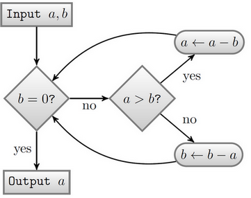
An algorithm is a sequence of instructions or rules to accomplish some task. An algorithm usually expects an input, and after performing a series of tasks on it, produces an output.
For example, the well-known Euclidean algorithm takes as input two natural numbers $a$ and $b$, and outputs the largest common divisor of $a$ and $b$.
A computer program is a sequence of coded instructions, written in a programming language, to be carried out by a computer. As such, a computer program is an implementation of an algorithm on a computer. There are many computer languages around, some of the more popular ones being C, C++, C#, Java, and Python. Computing platforms such as R, Julia, Sage or MATLAB also include their own programming languages. In this course we focus on Python. Some of the reasons are that it is
- easy to learn and use,
- comes with a large variety of libraries and add-ons for scientific computing and data science,
- is heavily used in organisations and industry, and many employers in quantitative and data-oriented fields expect applicants to know Python.
Below we see how the Euclidean algorithm looks like in Python.
a = int(input("Enter first number: "))
b = int(input("Enter second number: "))
while b != 0:
    if a > b:
        a = a - b
    else:
        b = b - a
print "The gcd of a and b is ", a
Enter first number: 38
Enter second number: 25
The gcd of a and b is  1
Remark 1: In this course we will be using Python 2.7, as opposed to Python 3.5. This is a subtle but important distinction, as some commands differe between the two version. The simple reason is that, for the time being, the optimization package CVXPY works best under Python 2.7.
Remark 2: This is a course on Convex Optimization and not on Python. We are only using Python as a computational tool to help us work with examples and applications related to optimization. For a more detailed introduction to Python, a good way to start is the Programming with Python (MATH20622) lecture, for which all the material is available online (note that the Python course is based on Python 3.5, but the differences are negligible). A comprehensive reference is the official Python Tutorial.
Jupyter
There are different ways to input Python code. One is entering the commands interactively using a command shell such as IPython. For larger software project, one typically uses an Integrated Development Environment (IDE), such as Spyder or PyCharm (there are countless others).
Jupyter notebooks can be seen as extensions of IPython. They are web applications that allow one to execute code written in Python (or other programming languages such as R and Julia), together with explanatory text, equations, web links, and media.
If you have a Python distribution such as Anaconda installed, then Jupyter is already there. Just go to the directory you like to work in and type "jupyter notebook" in a console (in Windows, type cmd to open a console). Otherwise, you can open or create a Jupyter notebook on your SageMathCloud account, see the instructions here for more details.
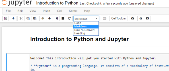
Jupyter notebooks contain two types of cells: Markdown and Code cells. Markdown cells are for writing text (this text is contained in a markdown cell!), while Code cells contain Python code. You can double-click on a cell and select the type of cell as follows:
In Markdown cells it is possible to format text (write section headers, enumerate, highlight text, etc). A reference on how how this is done can be found here. As with most things in life, the best way to learn is by doing, so I would encourage you to double-click on the markdown cells in this document and have a behind the scenes look at how this document was created. Once you finish writing a cell, you can move to the next one by typing SHIFT+ENTER. If you were in a Code cell, this will execute the code.
When working with Jupyter it is sometimes convenient to use keyboard shortcuts. A list can be found here.
Basic Python
The simplest program instructs the computer to print Hello World! on the screen. The \n command means newline, and tells the Python interpreter to "press enter" after outputting the text.
print "Hello World! \n"
Hello World!
Python can be used as a calculator to perform simple arithmetic. We can also add comments to the code by using the # sign. Comments are ignored by the interpreter, and serve only to make the code more readable.
# Add two numbers a and b and store the result in c
a = 2
b = 3
c = a+b
x = 2.7
y = x**2
print x, y
2.7 7.29
In the example above, a, b and c are variables, which store some data. In this case, they store the numbers 2, 3, and 2+3, respectively. We can change the values of variables any time.
a = a+4
# The following is a shortcut for b = b + 3 (similar with *,-,/)
b += 3
In Python we can make multiple assignments at the same time.
a, b, c = 1, 2, 3
print a, b, c
1 2 3
In Python we don't need to declare the type of data to be stored in a variable: it can be text, numbers, or other more complicated data types.
text = "I am a text string"
print text
I am a text string
You can add texts: what this does, is simpy join the different strings.
first = "Hello "
second = "World"
mystring = first + second + "!\n"
print mystring
Hello World!
You can also access individual letters. Indexing in Python starts with 0.
# Display the first 5 letters
print mystring[0:5]
# Display the last letter two letters. Note that the last letter is a newline character \n
print mystring[-2:-1]
Hello
!
A function takes inputs or arguments, and returns and output. In the above example, the function f is defined to take input values x and y and return the sum x+y.
Important: A feature that distinguishes Python from other programming languages is that it insists on indentation. Notice that the body of the function, everything that is carried out when the function is called, is indented: it is four characters (one 'tab') away from the left boundary. As soon as we are back on the left boundary, we are outside the function. The variable z appearing within the function is a local variable, it only exists while we are in the function. If we try to access it outside, we get an error.
Data types
Besides numbers and text strings, Python can deal with more involved data types. The most used one is the list.
# Lists
a = [1, 2, 3, 6]
b = ['hello', 3.1415, a]

# One can perform operations on list, like appending an element at the end
b.append('stop')
# the length of a list is given by len
print b, len(b)
['hello', 3.1415, [1, 2, 3, 6], 'stop'] 4
As seen in the above example, a list can contain arbitrary data types. List are indexed starting with 0. Thus if the list a has 4 elements, a[0] is the first and a[3] the last element. One can access various elements of a list using slicing.
# Print the second element of a
print a[1]
# Print the first three elements of c
print b[0:2]
# Print the last element of b
print b[-1]
2
['hello', 3.1415]
stop
A different data structure is the dictionary.
d = {'Item 1':1, 'Item 2':2}
d['Item 1']
1
In a dictionary, entries are labeled by a name and can be accessed that way.
Flow control and looping
Python, like most programming languages, can branch and carry out code subject to certain conditions being met. For example, in Euclide algorithm above, the computer encounters two numbers $a$ and $b$. If $a>b$, then it substracts $b$ from $a$, otherwise it subtracts $a$ from $b$.
n = input("Enter a number: ")
odd = n % 2
if odd:
    print "The number is odd."
else:
    print "The number is even."
Enter a number: 27
The number is odd.
x = int(input("Enter a number: "))
if x>5:
    print "The number is bigger than 5."
elif x<5:
    print "The number is smaller than 5."
else:
    print "The number is 5."
Enter a number: 8
The number is bigger than 5.
In the above code we used various constructs. "If odd" is a short for "If odd is 1", as "1" gets interpreted as True. The "else" applies if none of the conditions considered above apply.
Important: A feature that distinguishes Python from other programming languages is that it insists on indentation. Notice that everything that follows the if and elif statements is indented: it is four characters (one 'tab') away from the left boundary. As soon as we are back on the left boundary, we are outside the scope of the if or elif.
In programming, it is often necessary to repeat a task several times. For loops accomplish this. Python uses the command range(n) to list all the number from $0$ to $n-1$.
for i in range(5):
    print i**2
0
1
4
9
16
words = ['This', 'is', 'a', 'list', 'of', 'words', '.']
for w in words:
    print w
This
is
a
list
of
words
.
List comprehension means that we can concisely create lists using a for loop. The following contains the squares of the number 0 to 4.
squares = [x**2 for x in range(5)]
print squares
[0, 1, 4, 9, 16]
A related construction is the while loop: where, one repeats a task as long as some condition is met. Note that in each step, the values a and b are changed, so that eventually the validity of the condition may change.
a, b = 15, 5
while a>b:
    a = a - b
    print a
10
5
While loops can also be exited with a break command.
i = 0
while True:
    i += 1
    if i>10:
        break

print i
11
We finish the section on Basics with a short game from the Python lecture MATH20622. The commands available in Python are rather limited for more sophisticated applications. Luckily, there is the possibility of loading modules that provide additional features to the language. We will see a lot of modules below, the one we are using here is called random and the function that we load from this module is randint: it creates random numbers.
from random import randint  # Load the function randint from the module random

print "Guess a number between 1 and 100."
randomNumber = randint(1,100)  # Create a random number between 1 and 100
trials = 0                     # Record the number of trials

while True:                    # Repeat what follows until a 'break' command is encountered
    userGuess = int(input("Your guess: "))  # The 'int' converts the user input into an integer
    trials = trials + 1

    if userGuess == randomNumber:
        print "Hooray! It took you "+str(trials)+" trials."
        break
    else:
        print "Not correct!"
        if userGuess > randomNumber:
            print "Try a smaller number."
        else:
            print "Try a bigger number."
Guess a number between 1 and 100.
Your guess: 50
Not correct!
Try a smaller number.
Your guess: 25
Not correct!
Try a smaller number.
Your guess: 12
Not correct!
Try a bigger number.
Your guess: 19
Not correct!
Try a smaller number.
Your guess: 15
Not correct!
Try a bigger number.
Your guess: 17
Not correct!
Try a bigger number.
Your guess: 18
Hooray! It took you 7 trials.
Functions
In Python one can collect various tasks in functions, defined as follows.
def f(x,y):
    z = x + y
    return z

a = f(1,2)
print "The result of applying f is: ", a
The result of applying f is: 3
The variable z appearing within the function is a local variable, it only exists while we are in the function. If we try to access it outside, we get an error. It is also possible to pass arguments to a function as keywords, as in thefollowing example. Keywords can have a default value, that is used if the keyword or argument is not invoked.
def g(start, end=10):
    for i in range(start,end):
        print i

g(1)
print "\n"
g(3,end=7)
1
2
3
4
5
6
7
8
9


3
4
5
6
Numerical computing with Python
An important module or library is numpy, which stands for Numerical Python. To use numpy, one has to import it first. One could type **from numpy import * , which will import all command in numpy, but this is not recommended for efficiency reasons. Instead, one imports the numpy library using a short name np**, and one can then call all the numpy commands with the np. prefix (for example, np.sin(x) computes the sine of x).
import numpy as np
Numpy stores data in arrays. This include numbers, vectors, matrices, and higher order arrays. A matrix is interpreted as an array of arrays, as in the example below.
A = np.array([[1,2],[3,4]])
print A
[[1 2]
 [3 4]]
One can find information about the parameters of the array. For example, the following gives the shape (2 x 2). The L means that it stores the numbers in the "Long" format.
print A.shape
print A.ndim    # Prints the number of dimension. This is 2, because we are dealing with a matrix.
(2L, 2L)
2
numpy arrays carry a data type. If we want to work with floating point numbers, we should always add a decimal point to the numbers, otherwise Python will think they are integers. The type of data in a numpy array is determined by the dtype attribute.
A.dtype
dtype('int32')
Special matrices are the all zeros and all ones matrix, and the unit matrix.
B = np.zeros( (2,3) )
C = np.ones( (3,2) )
I = np.eye(2,2)
B[0,1], C[2,1]
(0.0, 1.0)
x = np.array([2, 3])
# Matrix vector product or matrix matrix product is implemented with np.dot
y = np.dot(A,x)
z = np.dot(C,I)
# The * operator
y_elementwise = A*x
print y, y_elementwise, z
[ 8 18] [[ 2  6]
 [ 6 12]] [[ 1.  1.]
 [ 1.  1.]
 [ 1.  1.]]
Plotting and graphics
Plotting is accomplished through the Matplotlib library. You can find a very good overview here. The following example illustrates the basic functionality.
import matplotlib.pyplot as plt
% matplotlib inline
# Create 100 points between 0 and 1
xx = np.linspace(0,1,100)
yy = np.exp(-2*xx)*np.sin(20*xx)
curve = plt.plot(xx,yy)

plt.title("Some curve")
plt.xlabel("x axis")
plt.ylabel("y axis")
plt.show()

# Save figure
plt.savefig("test.png")
<matplotlib.figure.Figure at 0x7801320>
We will often encounter contour plots of two-dimensional functions. As usual, the best way to learn to code is to read other code and examples, and a nice introduction to contour plots can be found here. Contour plots use what is known as a mesh grid. Given a range of x-values $(x_1,\dots,x_p)$ and y-values $(y_1,\dots,y_p)$, we want to evaluate a function $f(x_i,y_j)$ at all the pairs of points on the grid defined by the $x$ and $y$ values. For this purpose, one creates to matrices \begin{equation*} X = \begin{pmatrix} x_1 & x_2 & \cdots & x_p\\ x_1 & x_2 & \cdots & x_p\\ \vdots & \vdots & \ddots & \vdots\\ x_1 & x_2 & \cdots & x_p \end{pmatrix}, \quad Y = \begin{pmatrix} y_1 & y_1 & \cdots & y_1\\ y_2 & y_2 & \cdots & y_2\\ \vdots & \vdots & \ddots & \vdots\\ y_p & y_p & \cdots & y_p \end{pmatrix}. \end{equation*} Pairing each entrie of the $X$ matrix with the corresponding entry of the $Y$ matrix give every possible pair $(x_i,y_j)$. In Python (using the numpy module) one creates a meshgrid as follows.
xx = np.linspace(0,np.pi,100)   # Create a list of 100 points between 0 and Pi
yy = np.linspace(0,np.pi,100)
X, Y = np.meshgrid(xx,yy)
Next, define a function in two variables and apply this to the grid. The result of this is a matrix with the $f$-values for every pair $(x,y)$ with $x$ and $y$ from the lists created above.
def f(x,y):
    return np.sin(x*y)

Z = f(X,Y)
We can now apply matplotlib to create a contour plot.
plt.contourf(X,Y,Z)
plt.show()

There are other ways to generate contour plots, even in 3D. For more information, see the documentation.
CVXPY - Convex optimization in Python
For most computational experiments we will use the CVXPY package. This package usually has to be installed in addition to the Anaconda Python distribution, and the website gives instructions on how to do this. The example below shows how CVXPY can be used to solve a simple linear program. More involved examples appear in the first lecture.
import numpy as np
from cvxpy import *

# Problem data.
m = 30
n = 20
np.random.seed(1)
A = np.random.randn(m, n)
b = np.random.randn(m)

# Construct the problem.
x = Variable(n)
objective = Minimize(sum_squares(A*x - b))
constraints = [0 <= x, x <= 1]
prob = Problem(objective, constraints)

# The optimal objective is returned by prob.solve().
result = prob.solve()
# The optimal value for x is stored in x.value.
print x.value
# The optimal Lagrange multiplier for a constraint
# is stored in constraint.dual_value.
print constraints[0].dual_value
[[  2.74652308e-08]
 [  2.85638777e-02]
 [  2.75725989e-08]
 [  4.78319436e-08]
 [  2.63772742e-09]
 [  1.49296787e-01]
 [  1.19197012e-07]
 [  2.09644973e-08]
 [  2.46747598e-01]
 [  5.78236593e-01]
 [  5.29014714e-09]
 [  1.01716256e-03]
 [  8.73735490e-09]
 [  2.26771054e-01]
 [  1.37216315e-08]
 [  2.10136926e-08]
 [  4.08406457e-08]
 [  4.52408177e-09]
 [  2.55073731e-08]
 [  6.32803288e-09]]
[[  2.50930786e+00]
 [  2.67843812e-06]
 [  2.78353157e+00]
 [  1.79423617e+00]
 [  1.30858969e+01]
 [  5.59967336e-07]
 [  7.37035770e-01]
 [  3.35348867e+00]
 [  3.53776686e-07]
 [  1.58359789e-07]
 [  8.93824713e+00]
 [  3.08617390e-04]
 [  7.02959474e+00]
 [  3.97062919e-07]
 [  4.71054027e+00]
 [  3.18864113e+00]
 [  2.06076796e+00]
 [  1.00817336e+01]
 [  3.04814645e+00]
 [  8.53266394e+00]]
Other libraries
We will occasionally make use of other libraries.