Chapter 4. 모델 훈련
%matplotlib inline
import matplotlib
import matplotlib.pyplot as plt
plt.rcParams['axes.labelsize'] = 14
plt.rcParams['xtick.labelsize'] = 12
plt.rcParams['ytick.labelsize'] = 12
matplotlib.rc('font', family='NanumBarunGothic')
plt.rcParams['axes.unicode_minus'] = False

import os
import numpy as np
np.random.seed(42)

m = 100
X = 6 * np.random.rand(m, 1) - 3
y = 0.5 * X**2 + X + 2 + np.random.randn(m, 1)
4.4 학습곡선

from sklearn.metrics import mean_squared_error
from sklearn.model_selection import train_test_split
from sklearn.linear_model import LinearRegression

def plot_learning_curves(model, X, y):
    X_train, X_val, y_train, y_val = train_test_split(X, y, test_size=0.2, random_state=10)
    train_errors, val_errors = [], []
    print(X_train.shape, X_val.shape, y_train.shape, y_val.shape)
    for m in range(1, len(X_train)):
        model.fit(X_train[:m], y_train[:m])
        y_train_predict = model.predict(X_train[:m])
        y_val_predict = model.predict(X_val)
        train_errors.append(mean_squared_error(y_train[:m], y_train_predict))
        val_errors.append(mean_squared_error(y_val, y_val_predict))

    plt.plot(np.sqrt(train_errors), "r-+", linewidth=2, label="훈련")
    plt.plot(np.sqrt(val_errors), "b-", linewidth=3, label="검증")
    plt.legend(loc="upper right", fontsize=14)
    plt.xlabel("훈련 세트 크기", fontsize=14)
    plt.ylabel("RMSE", fontsize=14)

lin_reg = LinearRegression()
plot_learning_curves(lin_reg, X, y)
plt.axis([0, 80, 0, 3])
plt.show()
(80, 1) (20, 1) (80, 1) (20, 1)

▣ 단순 선형 회귀 모델(직선)의 학습 곡선
- 훈련 세트
- 샘플이 하나 혹은 두 개일 때는 모델이 완벽하게 작동
- 샘플이 추가됨에 따라 노이즈도 있고 데이터가 비선형이기 때문에 모델이 완벽히 학습하는 것이 불가능
- 오차가 계속 상승하다가 어느 정도를 유지
- 검증 세트
- 샘플의 수가 적으면 제대로 일반화될 수 없어서 검증 오차가 초기에 매우 큼
- 샘플이 추가됨에 따라 학습이 되고 검증 오차가 천천히 감소
- 선형 회귀의 직선은 데이터를 잘 모델링할 수 없으므로 오차의 감소가 완만해져서 훈련 세트의 그래프와 가까워짐
- 과소적합 모델의 전형적인 모습
→ 훈련 샘플을 더 추가해도 효과가 없음, 더 복잡한 모델을 사용하거나 더 나은 특성을 선택해야 함
▣ 10차 다항 회귀 모델의 학습 곡선
from sklearn.preprocessing import PolynomialFeatures
from sklearn.pipeline import Pipeline

polynomial_regression = Pipeline([
        ("poly_features", PolynomialFeatures(degree=10, include_bias=False)),
        ("lin_reg", LinearRegression()),
    ])

plot_learning_curves(polynomial_regression, X, y)
plt.axis([0, 80, 0, 3])
plt.show()
(80, 1) (20, 1) (80, 1) (20, 1)

- 훈련 데이터의 오차가 선형 회귀 모델보다 훨씬 낮음
- 두 곡선 사이에 공간이 있음. 훈련 데이터에서의 모델 성능이 검증 데이터에서보다 훨씬 낫다는 뜻으로 과대적합 모델의 특징임. 그러나 더 큰 훈련 세트를 사용하면 두 곡선이 점점 가까워짐
- 과대적합 모델을 개선하는 한 가지 방법은 검증 오차가 훈련 오차에 근접할 때까지 더 많은 훈련 데이터를 추가하는 것
▣ 편향/분산 트레이드오프
※ 모델의 일반화 오차는 세 가지 다른 종류의 오차의 합으로 표현할 수 있음
- 편향
일반화 오차 중에서 편향은 잘못된 가정으로 인한 것임. (예를 들어 데이터가 실제로는 2차인데 선형으로 가정하는 경우) 편향이 큰 모델은 훈련 데이터에 과소적합되기 쉬움
- 분산
분산variance은 훈련 데이터에 있는 작은 변동에 모델이 과도하게 민감하기 때문에 나타남. 자유도가 높은 모델(예를 들면 고차 다항 회귀 모델)이 높은 분산을 가지기 쉬워 훈련 데이터에 과대적합되는 경향이 있음
- 줄일 수 없는 오차
줄일 수 없는 오차irreducible error는 데이터 자체에 있는 노이즈 때문에 발생함. 이 오차를 줄일 수 있는 유일한 방법은 데이터에서 노이즈를 제거하는 것(예를 들어 고장 난 센서 같은 데이터 소스를 고치거나 이상치를 감지해 제거함)
※ 모델의 복잡도가 커지면 통상적으로 분산이 늘어나고 편향은 줄어듬. 반대로 모델의 복잡도가 줄어들면 편향이 커지고 분산이 작아짐.
4.5 규제가 있는 선형 모델
4.5.1 릿지 회귀
▣ 릿지 회귀(또는 티호노프Tikhonov 규제) : 규제가 추가된 선형 회귀
- 규제항 : 가중치 벡터의 $l_2$ 노름의 제곱을 2로 나눈 것을 사용
- $\alpha$로 모델을 얼마나 많이 규제할지 조절
- 규제항은 훈련하는 동안에만 비용 함수에 추가됨
- 모델의 훈련이 끝나면 모델의 성능을 규제가 없는 성능 지표로 평가

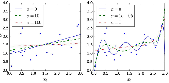
- 왼쪽 그래프는 평범한 릿지 모델
- 오른쪽 그래프는 PolynomialFeatures(degree=10)을 사용해 데이터를 확장하고 StandardScaler를 사용해 스케일을 조정한 릿지 모델
- $\alpha$가 커질수록 모든 가중치가 거의 0에 가까워지고 결국 데이터의 평균을 지나는 수평선이 됨
→ 모델의 분산은 줄지만 편향은 커짐
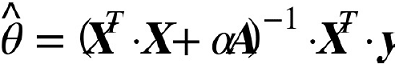
- A는 편향에 해당하는 맨 왼쪽 위의 원소가 0인 $(n+1)\times(n+1)$의 단위행렬identity matrix
from sklearn.linear_model import Ridge
from sklearn.linear_model import SGDRegressor

np.random.seed(42)
m = 20
X = 3 * np.random.rand(m, 1)
y = 1 + 0.5 * X + np.random.randn(m, 1) / 1.5
# 정규방정식을 사용한 릿지 회귀
ridge_reg = Ridge(alpha=1, solver="cholesky", random_state=42)
ridge_reg.fit(X, y)
ridge_reg.predict([[1.5]])
array([[1.55071465]])
- solver 매개변수의 기본값은 'auto'며 희소 행렬이나 특이 행렬(singular matrix)이 아닐 경우 'cholesky'가 됨
# 확률적 경사 하강법을 사용한 릿지 회귀
sgd_reg = SGDRegressor(max_iter=5, penalty="l2", random_state=42)
sgd_reg.fit(X, y.ravel())
sgd_reg.predict([[1.5]])
array([1.13500145])
ridge_reg = Ridge(alpha=1, solver="sag", random_state=42)
ridge_reg.fit(X, y)
ridge_reg.predict([[1.5]])
array([[1.5507201]])
- 확률적 평균 경사 하강법(Stochastic Average Gradient Descent, SAG) - SGD의 변종
: 현재 그래디언트와 이전 스텝에서 구한 모든 그래디언트를 합해서 평균한 값으로 모델 파라미터를 갱신
4.5.2 라쏘 회귀
▣ 라쏘Least Absolute and Selection Operator(Lasso) 회귀 : 선형 회귀의 또 다른 규제된 버전
- 규제항 : 가중치 벡터의 $l_1$ 노름을 사용


- 덜 중요한 특성의 가중치를 완전히 제거하려고 함(즉, 가중치가 0이 됨)
- 자동으로 특성 선택을 하고 희소 모델sparse model을 만듬(즉, 0이 아닌 특성의 가중치가 적음)

- 파란 배경의 등고선(타원형) : 규제가 없는($\alpha$=0) MSE 비용 함수
- 하얀색 원 : 비용 함수에 대한 배치 경사 하강법의 경로
- 무지개색 등고선 : $l_1$(다이아몬드형, 왼쪽 위), $l_2$(타원형, 왼쪽 아래) 페널티에 대한($\alpha$→∞) 배치 경사 하강법의 경로
- 오른쪽 위 그래프 : $\alpha$=0.5의 $l_1$ 페널티가 더해진 비용 함수 → 라쏘 회귀의 비용함수
- 오른쪽 아래 그래프 : $\alpha$=0.5의 $l_2$ 페널티가 더해진 비용 함수 → 릿지 회귀의 비용함수
※ 규제가 있는 경우의 최젓값이 규제가 없는 경우보다 $\theta$값이 0에 더 가까움(가중치가 완전히 제거되지는 않음)
- 라쏘의 비용 함수는 $\theta_i$=0($i$=1~n)에서 미분 불가능
→ 서브그래디언트 벡터subgradient vector g를 사용하여 해결

from sklearn.linear_model import Lasso

# 정규방정식을 사용한 라쏘 회귀
lasso_reg = Lasso(alpha=0.1)
lasso_reg.fit(X, y)
lasso_reg.predict([[1.5]])
array([1.53788174])
# 확률적 경사 하강법을 사용한 라쏘 회귀
sgd_reg = SGDRegressor(max_iter=5, penalty="l1", random_state=42)
sgd_reg.fit(X, y.ravel())
sgd_reg.predict([[1.5]])
array([1.13498188])
4.5.3 엘라스틱넷
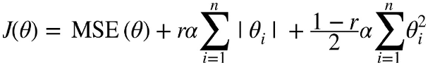
▣ 엘라스틱넷Elastic Net : 릿지 회귀와 라쏘 회귀를 절충한 모델
- 규제항은 릿지 회귀와 라쏘 회귀의 규제항을 단순히 더해서 사용
- 혼합 정도는 혼합 비율 r을 사용해 조절
- r=0 → 릿지 회귀
- r=1 → 라쏘 회귀
from sklearn.linear_model import ElasticNet

elastic_net = ElasticNet(alpha=0.1, l1_ratio=0.5, random_state=42)
elastic_net.fit(X, y)
elastic_net.predict([[1.5]])
array([1.54333232])
▣ 보통의 선형 회귀, 릿지, 라쏘, 엘라스틱넷
- 적어도 규제가 약간 있는 것이 대부분의 경우에 좋으므로 일반적으로 평범한 선형 회귀는 피해야 함
- 릿지가 기본, 실제로 쓰이는 특성이 몇 개뿐이라고 의심되면 라쏘나 엘라스틱넷이 좋음(불필요한 특성의 가중치를 0으로 만듦)
- 특성 수가 훈련 샘플 수보다 많거나 특성 몇 개가 강하게 연관되어 있을 때는 보통 라쏘보다 엘라스틱넷이 선호됨(라쏘는 특성 수가 샘플 수(n)보다 많으면 최대 n개의 특성을 선택함. 또, 여러 특성이 강하게 연관되어 있으면 이들 중 임의의 특성 하나를 선택함)
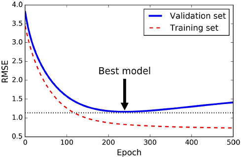
4.5.4 조기 종료
▣ 조기 종료early stopping : 검증 에러가 최솟값에 도달하면 바로 훈련을 중지시키는 방식
from sklearn.preprocessing import StandardScaler
from sklearn.base import clone

X_train, X_val, y_train, y_val = train_test_split(X[:50], y[:50].ravel(), test_size=0.5, random_state=10)

poly_scaler = Pipeline([
        ("poly_features", PolynomialFeatures(degree=90, include_bias=False)),
        ("std_scaler", StandardScaler()),
    ])

X_train_poly_scaled = poly_scaler.fit_transform(X_train)
X_val_poly_scaled = poly_scaler.transform(X_val)

sgd_reg = SGDRegressor(max_iter=1, warm_start=True, penalty=None,
                       learning_rate="constant", eta0=0.0005, random_state=42)

minimum_val_error = float("inf")
best_epoch = None
best_model = None
for epoch in range(1000):
    sgd_reg.fit(X_train_poly_scaled, y_train)  # 이어서 학습합니다
    y_val_predict = sgd_reg.predict(X_val_poly_scaled)
    val_error = mean_squared_error(y_val, y_val_predict)
    if val_error < minimum_val_error:
        minimum_val_error = val_error
        best_epoch = epoch
        best_model = clone(sgd_reg)

best_epoch, best_model
(287,
 SGDRegressor(alpha=0.0001, average=False, early_stopping=False, epsilon=0.1,
        eta0=0.0005, fit_intercept=True, l1_ratio=0.15,
        learning_rate='constant', loss='squared_loss', max_iter=1,
        n_iter=None, n_iter_no_change=5, penalty=None, power_t=0.25,
        random_state=42, shuffle=True, tol=None, validation_fraction=0.1,
        verbose=0, warm_start=True))
※ warm_start=True로 지정하면 fit() 메서드가 호출될 때 처음부터 다시 시작하지 않고 이전 모델 파라미터에서 훈련을 이어감
◈ SGDRegressor : https://scikit-learn.org/stable/modules/generated/sklearn.linear_model.SGDRegressor.html
4.6 로지스틱 회귀
▣ 로지스틱 회귀Logistic Regression(또는 로짓 회귀Logit Regression) : 샘플이 특정 클래스에 속할 확률을 추정
e.g.) 이메일이 스팸일 확률(이진 분류기)
4.6.1 확률 추정
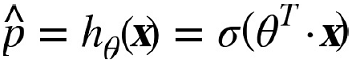
- ※ $\sigma(·)$ → logistic 또는 logit이라고 부름
- 0과 1사이의 값을 출력하는 시그모이드 함수sigmoid function (S자 형태)


4.6.2 훈련과 비용 함수


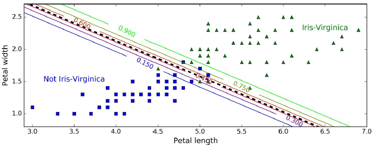
4.6.3 결정 경계
from sklearn import datasets

iris = datasets.load_iris()
list(iris.keys())
['feature_names', 'target_names', 'target', 'filename', 'data', 'DESCR']
iris.data.shape, iris.target.shape
((150, 4), (150,))
print(iris.DESCR)
.. _iris_dataset:

Iris plants dataset
--------------------

**Data Set Characteristics:**

    :Number of Instances: 150 (50 in each of three classes)
    :Number of Attributes: 4 numeric, predictive attributes and the class
    :Attribute Information:
        - sepal length in cm
        - sepal width in cm
        - petal length in cm
        - petal width in cm
        - class:
                - Iris-Setosa
                - Iris-Versicolour
                - Iris-Virginica

    :Summary Statistics:

    ============== ==== ==== ======= ===== ====================
                    Min  Max   Mean    SD   Class Correlation
    ============== ==== ==== ======= ===== ====================
    sepal length:   4.3  7.9   5.84   0.83    0.7826
    sepal width:    2.0  4.4   3.05   0.43   -0.4194
    petal length:   1.0  6.9   3.76   1.76    0.9490  (high!)
    petal width:    0.1  2.5   1.20   0.76    0.9565  (high!)
    ============== ==== ==== ======= ===== ====================

    :Missing Attribute Values: None
    :Class Distribution: 33.3% for each of 3 classes.
    :Creator: R.A. Fisher
    :Donor: Michael Marshall (MARSHALL%PLU@io.arc.nasa.gov)
    :Date: July, 1988

The famous Iris database, first used by Sir R.A. Fisher. The dataset is taken
from Fisher's paper. Note that it's the same as in R, but not as in the UCI
Machine Learning Repository, which has two wrong data points.

This is perhaps the best known database to be found in the
pattern recognition literature.  Fisher's paper is a classic in the field and
is referenced frequently to this day.  (See Duda & Hart, for example.)  The
data set contains 3 classes of 50 instances each, where each class refers to a
type of iris plant.  One class is linearly separable from the other 2; the
latter are NOT linearly separable from each other.

.. topic:: References

   - Fisher, R.A. "The use of multiple measurements in taxonomic problems"
     Annual Eugenics, 7, Part II, 179-188 (1936); also in "Contributions to
     Mathematical Statistics" (John Wiley, NY, 1950).
   - Duda, R.O., & Hart, P.E. (1973) Pattern Classification and Scene Analysis.
     (Q327.D83) John Wiley & Sons.  ISBN 0-471-22361-1.  See page 218.
   - Dasarathy, B.V. (1980) "Nosing Around the Neighborhood: A New System
     Structure and Classification Rule for Recognition in Partially Exposed
     Environments".  IEEE Transactions on Pattern Analysis and Machine
     Intelligence, Vol. PAMI-2, No. 1, 67-71.
   - Gates, G.W. (1972) "The Reduced Nearest Neighbor Rule".  IEEE Transactions
     on Information Theory, May 1972, 431-433.
   - See also: 1988 MLC Proceedings, 54-64.  Cheeseman et al"s AUTOCLASS II
     conceptual clustering system finds 3 classes in the data.
   - Many, many more ...
X = iris["data"][:, 3:]  # 꽃잎 넓이
y = (iris["target"] == 2).astype(np.int)  # Iris-Virginica이면 1 아니면 0

X.shape, y.shape
((150, 1), (150,))
from sklearn.linear_model import LogisticRegression

log_reg = LogisticRegression(solver='liblinear', random_state=42)
log_reg.fit(X, y)
LogisticRegression(C=1.0, class_weight=None, dual=False, fit_intercept=True,
          intercept_scaling=1, max_iter=100, multi_class='warn',
          n_jobs=None, penalty='l2', random_state=42, solver='liblinear',
          tol=0.0001, verbose=0, warm_start=False)
- 다른 선형 모델처럼 로지스틱 회귀 모델도 $l_1, l_2$ 페널티를 사용하여 규제할 수 있음
- 사이킷런은 $l_2$ 페널티를 기본으로 함
- LogisticRegression 모델의 규제 강도를 조절하는 하이퍼파라미터는
alpha가 아니고 그 역수에 해당하는 C(높을수록 규제가 줄어듦)
※ https://scikit-learn.org/stable/modules/generated/sklearn.linear_model.LogisticRegression.html
X_new = np.linspace(0, 3, 1000).reshape(-1, 1)
y_proba = log_reg.predict_proba(X_new)
decision_boundary = X_new[y_proba[:, 1] >= 0.5][0]

plt.figure(figsize=(8, 3))
plt.plot(X[y==0], y[y==0], "bs")
plt.plot(X[y==1], y[y==1], "g^")
plt.plot([decision_boundary, decision_boundary], [-1, 2], "k:", linewidth=2)
plt.plot(X_new, y_proba[:, 1], "g-", linewidth=2, label="Iris-Virginica")
plt.plot(X_new, y_proba[:, 0], "b--", linewidth=2, label="Not Iris-Virginica")
plt.text(decision_boundary+0.02, 0.15, "결정 경계", fontsize=14, color="k", ha="center")
plt.arrow(decision_boundary, 0.08, -0.3, 0, head_width=0.05, head_length=0.1, fc='b', ec='b')
plt.arrow(decision_boundary, 0.92, 0.3, 0, head_width=0.05, head_length=0.1, fc='g', ec='g')
plt.xlabel("꽃잎의 폭 (cm)", fontsize=14)
plt.ylabel("확률", fontsize=14)
plt.legend(loc="center left", fontsize=14)
plt.axis([0, 3, -0.02, 1.02])
plt.show()

decision_boundary
array([1.61561562])
log_reg.predict([[1.7], [1.5]])
array([1, 0])
4.6.4 소프트맥스 회귀
▣ 소프트맥스 회귀softmax Regression 또는 다항 로지스틱 회귀Multinomial Logistic Regression
- 각 클래스는 자신만의 파라미터 벡터 $\theta^{(k)}$가 있음
- 이 벡터들은 파라미터 행렬parameter matrix $\Theta$에 행으로 저장됨

- K는 클래스 수
- $s(x)$는 샘플 x에 대한 각 클래스의 점수를 담고 있는 벡터
- $\sigma(s(x))_k$는 샘플 x에 대한 각 클래스의 점수가 주어졌을 때 이 샘플이 클래스 k에 속할 추정 확률

- 추정 확률이 가장 높은 클래스 → 가장 높은 점수를 가진 클래스
※ 소프트맥스 회귀 분류기는 다중 출력multioutput이 아니라 한 번에 하나의 클래스만 예측하는 다중 클래스multiclass이기 때문에 상호 배타적인 클래스에서만 사용해야 함
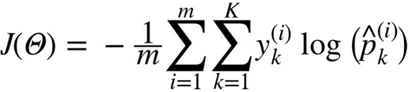
- $i$번째 샘플에 대한 타깃 클래스가 $k$일 때 $y_k^{(i)}$가 1이고, 그 외에는 0
- 딱 두 개의 클래스가 있을 때(K=2) 이 비용 함수는 로지스틱 회귀의 비용 함수와 같음(식 4-17의 로그 손실)
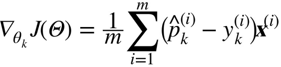
X = iris["data"][:, (2, 3)]  # 꽃잎 길이, 꽃잎 넓이
y = iris["target"]

softmax_reg = LogisticRegression(multi_class="multinomial",solver="lbfgs", C=10, random_state=42)
softmax_reg.fit(X, y)
LogisticRegression(C=10, class_weight=None, dual=False, fit_intercept=True,
          intercept_scaling=1, max_iter=100, multi_class='multinomial',
          n_jobs=None, penalty='l2', random_state=42, solver='lbfgs',
          tol=0.0001, verbose=0, warm_start=False)
- LogisticRegression은 클래스가 둘 이상일 때 기본적으로 일대다(OvA) 전략을 사용
- multi_class 매개변수를 "multinomial"로 바꾸면 소프트맥스 회귀를 사용할 수 있음
- 소프트맥스 회귀를 사용하려면 solver 매개변수에 "lbfgs"와 같이 소프트맥스 회귀를 지원하는 알고리즘을 지정해야 함
softmax_reg.predict([[5, 2]])
array([2])
softmax_reg.predict_proba([[5, 2]])
array([[6.38014896e-07, 5.74929995e-02, 9.42506362e-01]])
4.7 연습문제
1. 수백만 개의 특성을 가진 훈련 세트에서는 어떤 선형 회귀 알고리즘을 사용할 수 있을까요?
☞ 수백만 개의 특성이 있는 훈련 세트를 가지고 있다면 확률적 경사 하강법(SGD)이나 미니배치 경사하강법을 사용할 수 있습니다. 훈련 세트가 메모리 크기에 맞으면 배치 경사 하강법도 가능합니다. 하지만 정규방정식은 계산 복잡도가 특성 개수에 따라 매우 빠르게 증가하기 때문에 사용할 수 없습니다.
2. 훈련 세트에 있는 특성들이 각기 아주 다른 스케일을 가지고 있습니다. 이런 데이터에 잘 작동하지 않는 알고리즘은 무엇일까요? 그 이유는 무엇일까요? 이 문제를 어떻게 해결할 수 있을까요?
☞ 훈련 세트에 있는 특성의 스케일이 매우 다르면 비용 함수는 길쭉한 타원 모양의 그릇 형태가 됩니다. 그래서 경사 하강법(GD) 알고리즘이 수렴하는 데 오랜 시간이 걸릴 것입니다. 이를 해결하기 위해서는 모델을 훈련하기 전에 데이터의 스케일을 조절해야 합니다. 정규방정식은 스케일 조정 없이도 잘 작동합니다. 또한 규제가 있는 모델은 특성의 스케일이 다르면 지역 최적점에 수렴할 가능성이 있습니다. 실제로 규제는 가중치가 커지지 못하게 제약을 가하므로 특성값이 작으면 큰 값을 가진 특성에 비해 무시되는 경향이 있습니다.
3. 경사 하강법으로 로지스틱 회귀 모델을 훈련시킬 때 지역 최솟값에 갇힐 가능성이 있을까요?
☞ 로지스틱 회귀 모델의 비용 함수는 볼록 함수이므로 경사 하강법이 훈련될 때 지역 최솟값에 갇힐 가능성이 없습니다.
4. 충분히 오랫동안 실행하면 모든 경사 하강법 알고리즘이 같은 모델을 만들어낼까요?
☞ 최적화할 함수가 (선형 회귀나 로지스틱 회귀처럼) 볼록 함수이고 학습률이 너무 크지 않다고 가정하면 모든 경사 하강법 알고리즘이 전역 최적값에 도달하고 결국 비슷한 모델을 만들 것입니다. 하지만 학습률을 점진적으로 감소시키지 않으면 SGD와 미니배치 GD는 진정한 최적점에 수렴하지 못할 것입니다. 대신 전역 최적점 주변을 이리저리 맴돌게 됩니다. 이 말은 매우 오랫동안 훈련을 해도 경사 하강법 알고리즘들은 조금씩 다른 모델을 만들게 된다는 뜻입니다.
5. 배치 경사 하강법을 사용하고 에포크마다 검증 오차를 그래프로 나타내봤습니다. 검증 오차가 일정하게 상승되고 있다면 어떤 일이 일어나고 있는 걸까요? 이 문제를 어떻게 해결할 수 있나요?
- 훈련 에러도 같이 올라간다면 학습률이 너무 높아 알고리즘이 발산하는 것이기 때문에 학습률을 낮추어야 함
- 훈련 에러는 올라가지 않는다면 모델이 훈련 세트에 과대적합된 것이므로 훈련을 멈추어야 함
6. 검증 오차가 상승하면 미니배치 경사 하강법을 즉시 중단하는 것이 좋은 방법인가요?
☞ 무작위성 때문에 확률적 경사 하강법이나 미니배치 경사 하강법 모두 매 훈련 반복마다 학습의 진전을 보장하지 못합니다. 검증 에러가 상승될 때 훈련을 즉시 멈춘다면 최적점에 도달하기 전에 너무 일찍 멈추게 될지 모릅니다. 더 나은 방법은 정기적으로 모델을 저장하고 오랫동안 진전이 없을 때(즉, 최상의 점수를 넘어서지 못하면), 저장된 것 중 가장 좋은 모델로 복원하는 것입니다.
7. (우리가 언급한 것 중에서) 어떤 경사 하강법 알고리즘이 가장 빠르게 최적 솔루션의 주변에 도달할까요? 실제로 수렴하는 것은 어떤 것인가요? 다른 방법들도 수렴하게 만들 수 있나요?
☞ 확률적 경사 하강법은 한 번에 하나의 훈련 샘플만 사용하기 때문에 훈련 반복이 가장 빠릅니다. 그래서 가장 먼저 전역 최적점 근처에 도달합니다(그다음이 작은 미니배치 크기를 가진 미니배치 GD입니다). 그러나 훈련 시간이 충분하면 배치 경사 하강법만 실제로 수렴할 것입니다. 앞서 언급한 대로 학습률을 점진적으로 감소시키지 않으면 SGD와 미니배치 GD는 최적점 주변을 맴돌 것입니다.
8. 다항 회귀를 사용했을 때 학습 곡선을 보니 훈련 오차와 검증 오차 사이에 간격이 큽니다. 무슨 일이 생긴 걸까요? 이 문제를 해결하는 세 가지 방법은 무엇인가요?
☞ 검증 오차가 훈련 오차보다 훨씬 더 높으면 모델이 훈련 세트에 과대적합되었기 때문일 가능성이 높습니다.
- 다항 차수 낮추기 : 자유도를 줄이면 과대적합이 훨씬 줄어들 것임
- 모델을 규제 : 예를 들어 비용 함수에 $l_2$ 페널티(릿지)나 $l_1$ 페널티(라쏘)를 추가(이 방법도 모델의 자유도를 감소시킴)
- 훈련 세트의 크기 증가시키기
9. 릿지 회귀를 사용했을 때 훈련 오차와 검증 오차가 거의 비슷하고 둘 다 높았습니다. 이 모델에는 높은 편향이 문제인가요, 아니면 높은 분산이 문제인가요? 규제 하이퍼파라미터 $\alpha$를 증가시켜야 할까요, 아니면 줄여야 할까요?
☞ 훈련 에러와 검증 에러가 거의 비슷하고 매우 높다면 모델이 훈련 세트에 과소적합되었을 가능성이 높습니다. 즉, 높은 편향을 가진 모델입니다. 따라서 규제 하이퍼파라미터 $\alpha$를 감소시켜야 합니다.
10. 다음과 같이 사용해야 하는 이유는?
- 평범한 선형 회귀(즉, 아무런 규제가 없는 모델) 대신 릿지 회귀
- 릿지 회귀 대신 라쏘 회귀
- 라쏘 회귀 대신 엘라스틱넷
- 규제가 있는 모델이 일반적으로 규제가 없는 모델보다 성능이 좋습니다. 그래서 평범한 선형 회귀보다 릿지 회귀가 선호됩니다.
- 라쏘 회귀는 $l_1$ 페널티를 사용하여 가중치를 완전히 0으로 만드는 경향이 있습니다. 이는 가장 중요한 가중치를 제외하고는 모두 0이 되는 희소한 모델을 만듭니다. 또한 자동으로 특성 선택의 효과를 가지므로 단지 몇 개의 특성만 실제 유용할 것이라고 의심될 때 사용하면 좋습니다. 만약 확신이 없다면 릿지 회귀를 사용해야 합니다.
- 라쏘가 어떤 경우(몇 개의 특성이 강하게 연관되어 있거나 훈련 샘플보다 특성이 더 많을 때)에는 불규칙하게 행동하므로 엘라스틱넷이 라쏘보다 일반적으로 선호됩니다. 그러나 추가적인 하이퍼파라미터가 생깁니다. 불규칙한 행동이 없는 라쏘를 원하면 엘라스틱넷에 l1_ratio를 1에 가깝게 설정하면 됩니다.
11. 사진을 낮과 밤, 실내와 실외로 분류하려 합니다. 두 개의 로지스틱 회귀 분류기를 만들어야 할까요, 아니면 하나의 소프트맥스 회귀 분류기를 만들어야 할까요?
☞ 실외와 실내, 낮과 밤에 따라 사진을 구분하고 싶다면 이 둘은 배타적인 클래스가 아니기 때문에(즉, 네 가지 조합이 모두 가능하므로) 두 개의 로지스틱 회귀 분류기를 훈련시켜야 합니다.