Chapter 2. 머신러닝 프로젝트 처음부터 끝까지
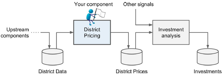
◈ 진행할 주요 단계(부동산 회사라 가정)
- 큰 그림을 본다.
- 데이터를 구한다.
- 데이터로부터 통찰을 얻기 위해 탐색하고 시각화한다.
- 머신러닝 알고리즘을 위해 데이터를 준비한다.
- 모델을 선택하고 훈련시킨다.
- 모델을 상세하게 조정한다.
- 솔루션을 제시한다.
- 시스템을 론칭하고 모니터링하고 유지 보수한다.
2.1 실제 데이터로 작업하기
- 유명한 공개 데이터 저장소
- UC 얼바인Irvine 머신러닝 저장소(http://archive.ics.uci.edu/ml/)
- 캐글Kaggle 데이터셋(http://www.kaggle.com/datasets)
- 아마존 AWS 데이터셋(http://aws.amazon.com/ko/datasets)
- 메타 포털(공개 데이터 저장소가 나열되어 있음)
- 인기 있는 공개 데이터 저장소가 나열되어 있는 다른 페이지
- 위키백과 머신러닝 데이터셋 목록(http://goo.gl/SJHN2k)
- Quora.com 질문(http://goo.gl/zDR78y)
- 데이터셋 서브레딧subreddit(http://www.reddit.com/r/datasets)

2.2 큰 그림 보기
2.2.1 문제 정의
▣비즈니스의 정확한 목적?(이익을 어떻게 얻을지)
- 문제 정의(알고리즘 선택)
- 모델 평가
- 모델 튜닝
■ 문제 정의
- Training Set에 레이블(중간 주택 가격)이 있음 → 지도 학습
- 값(중간 주택 가격)을 예측해야 함 → 회귀
- 예측에 사용할 특성이 여러 개(구역의 인구, 중간 소득 등) → 다변량 회귀multivariate regression (특성이 한 개라면 단변량 회귀univariate regression)
- 빠르게 변하는 데이터에 적응하지 않아도 되고, 데이터가 메모리에 들어갈 만큼 충분히 작음 → 배치 학습
2.2.2 성능 측정 지표 선택
▶평균 제곱근 오차Root Mean Square Error(RMSE)
- 유클리디안 노름Euclidian norm
- 회귀 문제의 전형적인 성능 지표
- 오차가 커질수록 값이 더욱 커짐
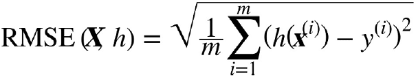
- m → RMSE를 측정할 데이터셋에 있는 샘플 수
- x(i) → i번째 샘플의 전체 특성값(레이블은 제외)의 벡터
- y(i) → i번째 샘플의 레이블(기대 출력값)
- X → 데이터셋에 있는 모든 샘플의 모든 특성값(레이블은 제외)을 포함하는 행렬
- h → 가설hypothesis
- RMSE(X, h) → 가설 h를 사용하여 일련의 샘플을 평가하는 비용 함수
▶평균 절대 오차Mean Absolute Error(MAE)
- 맨해튼 노름Manhattan norm
- 이상치가 많을 때
- RMSE와 MAE 모두 예측값의 벡터와 타깃값의 벡터 사이의 거리를 재는 방법

2.2.3 가정 검사
- 지금까지 만든 가정을 나열하고 검사
2.3 데이터 가져오기
2.3.1 작업환경 만들기
▶아나콘다(Anaconda) 설치
$ conda create -n mlbook python=3.5 anaconda
$ activate mlbook
$ conda install -n mlbook -c conda-forge tensorflow
$ jupyter notebook
2.3.2 데이터 다운로드
▶깃허브
https://github.com/rickiepark/handson-ml
/hands_on_ml_link/datasets/housing/housing.csv
import os
import pandas as pd

HOUSING_PATH = os.path.join("datasets", "housing")

def load_housing_data(housing_path=HOUSING_PATH):
    csv_path = os.path.join(housing_path, "housing.csv")
    return pd.read_csv(csv_path)
- 이 함수는 모든 데이터를 담은 판다스의 데이터프레임 객체를 반환
2.3.3 데이터 구조 훑어보기
housing = load_housing_data()
housing.head()
| longitude | latitude | housing_median_age | total_rooms | total_bedrooms | population | households | median_income | median_house_value | ocean_proximity | |
|---|---|---|---|---|---|---|---|---|---|---|
| 0 | -122.23 | 37.88 | 41.0 | 880.0 | 129.0 | 322.0 | 126.0 | 8.3252 | 452600.0 | NEAR BAY |
| 1 | -122.22 | 37.86 | 21.0 | 7099.0 | 1106.0 | 2401.0 | 1138.0 | 8.3014 | 358500.0 | NEAR BAY |
| 2 | -122.24 | 37.85 | 52.0 | 1467.0 | 190.0 | 496.0 | 177.0 | 7.2574 | 352100.0 | NEAR BAY |
| 3 | -122.25 | 37.85 | 52.0 | 1274.0 | 235.0 | 558.0 | 219.0 | 5.6431 | 341300.0 | NEAR BAY |
| 4 | -122.25 | 37.85 | 52.0 | 1627.0 | 280.0 | 565.0 | 259.0 | 3.8462 | 342200.0 | NEAR BAY |
- 데이터셋의 처음 다섯 행
- 각 행은 하나의 구역을 나타냄
housing.info()
<class 'pandas.core.frame.DataFrame'>
RangeIndex: 20640 entries, 0 to 20639
Data columns (total 10 columns):
longitude             20640 non-null float64
latitude              20640 non-null float64
housing_median_age    20640 non-null float64
total_rooms           20640 non-null float64
total_bedrooms        20433 non-null float64
population            20640 non-null float64
households            20640 non-null float64
median_income         20640 non-null float64
median_house_value    20640 non-null float64
ocean_proximity       20640 non-null object
dtypes: float64(9), object(1)
memory usage: 1.6+ MB
- 각 특성의 데이터 타입
- 전체 행 수(전체 샘플 수)
- 각 특성의 널null이 아닌 값의 개수
housing["ocean_proximity"].value_counts()
<1H OCEAN     9136
INLAND        6551
NEAR OCEAN    2658
NEAR BAY      2290
ISLAND           5
Name: ocean_proximity, dtype: int64
- CSV 파일에서 읽어 들였기 때문에 텍스트 특성
- 범주형categorical
housing.describe()
| longitude | latitude | housing_median_age | total_rooms | total_bedrooms | population | households | median_income | median_house_value | |
|---|---|---|---|---|---|---|---|---|---|
| count | 20640.000000 | 20640.000000 | 20640.000000 | 20640.000000 | 20433.000000 | 20640.000000 | 20640.000000 | 20640.000000 | 20640.000000 |
| mean | -119.569704 | 35.631861 | 28.639486 | 2635.763081 | 537.870553 | 1425.476744 | 499.539680 | 3.870671 | 206855.816909 |
| std | 2.003532 | 2.135952 | 12.585558 | 2181.615252 | 421.385070 | 1132.462122 | 382.329753 | 1.899822 | 115395.615874 |
| min | -124.350000 | 32.540000 | 1.000000 | 2.000000 | 1.000000 | 3.000000 | 1.000000 | 0.499900 | 14999.000000 |
| 25% | -121.800000 | 33.930000 | 18.000000 | 1447.750000 | 296.000000 | 787.000000 | 280.000000 | 2.563400 | 119600.000000 |
| 50% | -118.490000 | 34.260000 | 29.000000 | 2127.000000 | 435.000000 | 1166.000000 | 409.000000 | 3.534800 | 179700.000000 |
| 75% | -118.010000 | 37.710000 | 37.000000 | 3148.000000 | 647.000000 | 1725.000000 | 605.000000 | 4.743250 | 264725.000000 |
| max | -114.310000 | 41.950000 | 52.000000 | 39320.000000 | 6445.000000 | 35682.000000 | 6082.000000 | 15.000100 | 500001.000000 |
- 숫자형 특성의 요약 정보
- std → 표준편차
- 25%, 50%, 75% → 백분위수percentile : 전체 관측값에서 주어진 백분율이 속하는 하위 부분의 값
%matplotlib inline
import matplotlib.pyplot as plt
housing.hist(bins=50, figsize=(20,15))
plt.show()

- 모든 숫자형 특성에 대한 히스토그램
- 주어진 값의 범위(수평축)에 속한 샘플 수(수직축)를 나타냄
2.3.4 테스트 세트 만들기
- 데이터 스누핑data snooping 편향 : 만약 테스트 세트를 들여다본다면 테스트 세트에서 겉으로 드러난 어떤 패턴에 속아 특정 머신러닝 모델을 선택하게 될지도 모름, 이 테스트 세트로 일반화 오차를 추정하면 매우 낙관적인 추정이 되며 시스템을 론칭했을 때 기대한 성능이 나오지 않을 것임
import numpy as np

def split_train_test(data, test_ratio):
    shuffled_indices = np.random.permutation(len(data))
    test_set_size = int(len(data) * test_ratio)
    test_indices = shuffled_indices[:test_set_size]
    train_indices = shuffled_indices[test_set_size:]
    return data.iloc[train_indices], data.iloc[test_indices]

train_set, test_set = split_train_test(housing, 0.2)
print(len(train_set), "train +", len(test_set), "test")
16512 train + 4128 test
- 무작위로 전체 데이터셋의 20%를 테스트 세트로 분리
- 프로그램을 다시 실행하면 다른 테스트 세트가 생성됨 (→ 여러 번 반복하면 데이터 스누핑)
np.random.permutation(10)
array([9, 6, 4, 5, 8, 7, 1, 0, 2, 3])
housing.iloc[[32, 627, 2373]]
| longitude | latitude | housing_median_age | total_rooms | total_bedrooms | population | households | median_income | median_house_value | ocean_proximity | |
|---|---|---|---|---|---|---|---|---|---|---|
| 32 | -122.27 | 37.84 | 48.0 | 1922.0 | 409.0 | 1026.0 | 335.0 | 1.7969 | 110400.0 | NEAR BAY |
| 627 | -122.18 | 37.70 | 35.0 | 2562.0 | 554.0 | 1398.0 | 525.0 | 3.3906 | 178900.0 | NEAR BAY |
| 2373 | -119.57 | 36.70 | 30.0 | 2370.0 | 412.0 | 1248.0 | 410.0 | 3.1442 | 72300.0 | INLAND |
from sklearn.model_selection import train_test_split

train_set, test_set = train_test_split(housing, test_size=0.2, random_state=42)
- 난수 초깃값을 지정할 수 있어서 프로그램을 다시 실행해도 같은 테스트 세트가 생성됨(동일한 데이터셋을 사용한다면)
- 데이터셋이 업데이트가 되는 경우에는 각 샘플마다 식별자의 해시값을 활용하여 테스트 세트를 유지할 수 있음
▷무작위 샘플링 방식은 특성 수에 비해 데이터셋이 충분히 크다면 일반적으로 괜찮지만, 그렇지 않다면 샘플링 편향이 생길 가능성이 큼
▶계층적 샘플링stratified sampling : 전체 모수는 계층strata이라는 동질의 그룹으로 나뉘고, 테스트 세트가 전체 모수를 대표하도록 각 계층에서 올바른 수의 샘플을 추출하는 것
- 계층별로 데이터셋에 충분한 샘플 수가 있어야 함(그렇지 않으면 편향이 발생)
- 너무 많은 계층으로 나누면 안 됨
housing["income_cat"] = np.ceil(housing["median_income"] / 1.5) # 소득의 카테고리 수를 제한(나누기), 이산적인 카테고리 만들기(올림)
housing["income_cat"].where(housing["income_cat"] < 5, 5.0, inplace=True)
s = pd.Series(range(5))
s.where(s > 1, 10)
0    10
1    10
2     2
3     3
4     4
dtype: int64
housing["income_cat"].hist()
<matplotlib.axes._subplots.AxesSubplot at 0x227af071e80>

from sklearn.model_selection import StratifiedShuffleSplit

split = StratifiedShuffleSplit(n_splits=1, test_size=0.2, random_state=42) # n_splits = Number of re-shuffling & splitting iterations.
for train_index, test_index in split.split(housing, housing["income_cat"]):
    # print(train_index, test_index)
    strat_train_set = housing.loc[train_index]
    strat_test_set = housing.loc[test_index]
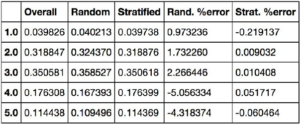
# 전체 주택 데이터셋에서 소득 카테고리의 비율
housing["income_cat"].value_counts() / len(housing)
3.0    0.350581
2.0    0.318847
4.0    0.176308
5.0    0.114438
1.0    0.039826
Name: income_cat, dtype: float64
# 테스트 주택 데이터셋에서 소득 카테고리의 비율(무작위 샘플링)
train_set, test_set = train_test_split(housing, test_size=0.2, random_state=42)
test_set["income_cat"].value_counts() / len(test_set)
3.0    0.358527
2.0    0.324370
4.0    0.167393
5.0    0.109496
1.0    0.040213
Name: income_cat, dtype: float64
# 테스트 주택 데이터셋에서 소득 카테고리의 비율(계층 샘플링)
strat_test_set["income_cat"].value_counts() / len(strat_test_set)
3.0    0.350533
2.0    0.318798
4.0    0.176357
5.0    0.114583
1.0    0.039729
Name: income_cat, dtype: float64
for set_ in (strat_train_set, strat_test_set):
    set_.drop("income_cat", axis=1, inplace=True)
2.4 데이터 이해를 위한 탐색과 시각화
# 훈련 세트를 손상시키지 않기 위해 복사본 생성
housing = strat_train_set.copy()
2.4.1 지리적 데이터 시각화
housing.plot(kind="scatter", x="longitude", y="latitude")
<matplotlib.axes._subplots.AxesSubplot at 0x227af6c67b8>

- 데이터의 지리적인 산점도
housing.plot(kind="scatter", x="longitude", y="latitude", alpha=0.1)
<matplotlib.axes._subplots.AxesSubplot at 0x227af136240>

housing.plot(kind="scatter", x="longitude", y="latitude", alpha=0.4,
            s=housing["population"]/100, label="population", figsize=(10,7),
            c="median_house_value", cmap=plt.get_cmap("jet"), colorbar=True, sharex=False)
plt.legend()
<matplotlib.legend.Legend at 0x227af0ee8d0>

- 캘리포니아 중간 주택 가격
- s(원의 반지름) → 구역의 인구
- c(색깔) → 가격
- cmap("jet") → 파란색(낮은 가격) ~ 빨간색(높은 가격)
2.4.2 상관관계 조사
- 데이터셋이 크지 않으므로 모든 특성 간의 표준 상관계수standard correlation coefficient (피어슨의 *r*이라고도 부름)를 corr() 메소드를 이용해 쉽계 계산할 수 있음
corr_matrix = housing.corr()
# 중간 주택 가격과 다른 특성 사이의 상관관계 크기
corr_matrix["median_house_value"].sort_values(ascending=False)
median_house_value    1.000000
median_income         0.687160
total_rooms           0.135097
housing_median_age    0.114110
households            0.064506
total_bedrooms        0.047689
population           -0.026920
longitude            -0.047432
latitude             -0.142724
Name: median_house_value, dtype: float64
- 범위는 -1 ~ 1
- 1에 가까울수록 강한 양의 상관관계
- -1에 가까울수록 강한 음의 상관관계
- 0에 가까우면 선형적인 상관관계가 없음
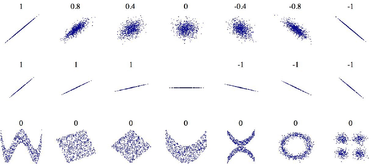
- 상관계수는 선형적인 상관관계(x가 증가하면 y는 증가하거나 감소)만 측정함 → 상관계수는 기울기와 상관없음
- 비선형적인 관계는 잡을 수 없음 → 마지막 줄에 있는 그래프들은 두 축이 완전히 독립적이지 않음에도 상관계수가 0
# 숫자형 특성 사이에 산점도를 그려주는 판다스의 scatter_matrix 함수
from pandas.plotting import scatter_matrix

attributes = ["median_house_value", "median_income", "total_rooms", "housing_median_age"]
scatter_matrix(housing[attributes], figsize=(12, 8))
array([[<matplotlib.axes._subplots.AxesSubplot object at 0x00000227B1335E10>,
        <matplotlib.axes._subplots.AxesSubplot object at 0x00000227B11EF278>,
        <matplotlib.axes._subplots.AxesSubplot object at 0x00000227B1205908>,
        <matplotlib.axes._subplots.AxesSubplot object at 0x00000227B1220F98>],
       [<matplotlib.axes._subplots.AxesSubplot object at 0x00000227B123C668>,
        <matplotlib.axes._subplots.AxesSubplot object at 0x00000227B1255CF8>,
        <matplotlib.axes._subplots.AxesSubplot object at 0x00000227B12733C8>,
        <matplotlib.axes._subplots.AxesSubplot object at 0x00000227B128AA58>],
       [<matplotlib.axes._subplots.AxesSubplot object at 0x00000227B12A9128>,
        <matplotlib.axes._subplots.AxesSubplot object at 0x00000227B12C07B8>,
        <matplotlib.axes._subplots.AxesSubplot object at 0x00000227B12DAE48>,
        <matplotlib.axes._subplots.AxesSubplot object at 0x00000227B12F7518>],
       [<matplotlib.axes._subplots.AxesSubplot object at 0x00000227B130FBA8>,
        <matplotlib.axes._subplots.AxesSubplot object at 0x00000227B136E278>,
        <matplotlib.axes._subplots.AxesSubplot object at 0x00000227B1386908>,
        <matplotlib.axes._subplots.AxesSubplot object at 0x00000227B139FF98>]],
      dtype=object)

- 각 변수 자신에 대한 그래프는 의미없는 직선이 나오므로 판다스는 이곳에 각 특성의 히스토그램을 그림
- 중간 주택 가격(median_house_value)을 예측하는 데 가장 유용할 것 같은 특성은 중간 소득(median_income)
housing.plot(kind="scatter", x="median_income", y="median_house_value", alpha=0.1)
<matplotlib.axes._subplots.AxesSubplot at 0x227b1694f98>

- 상관관계가 매우 강함(위쪽으로 향하는 경향) : 포인트들이 너무 널리 퍼져 있지 않음
- 가격 제한 값($500,000)이 잘 보임
2.4.3 특성 조합으로 실험
housing["rooms_per_household"] = housing["total_rooms"] / housing["households"]
housing["bedrooms_per_room"] = housing["total_bedrooms"] / housing["total_rooms"]
housing["population_per_household"] = housing["population"] / housing["households"]

corr_matrix = housing.corr()
corr_matrix["median_house_value"].sort_values(ascending=False)
median_house_value          1.000000
median_income               0.687160
rooms_per_household         0.146285
total_rooms                 0.135097
housing_median_age          0.114110
households                  0.064506
total_bedrooms              0.047689
population_per_household   -0.021985
population                 -0.026920
longitude                  -0.047432
latitude                   -0.142724
bedrooms_per_room          -0.259984
Name: median_house_value, dtype: float64
2.5 머신러닝 알고리즘을 위한 데이터 준비
▣ 데이터 준비를 함수로 자동화해야 하는 이유
- 어떤 데이터셋에 대해서도 데이터 변환을 손쉽게 반복할 수 있다 (e.g. 다음번에 새로운 데이터셋을 사용할 때)
- 향후 프로젝트에 사용할 수 있는 변환 라이브러리를 점진적으로 구축하게 된다
- 실제 시스템에서 알고리즘에 새 데이터를 주입하기 전에 변환시키는 데 이 함수를 사용할 수 있다
- 여러 가지 데이터 변환을 쉽게 시도해볼 수 있고 어떤 조합이 가장 좋은지 확인하는 데 편리하다
housing = strat_train_set.drop("median_house_value", axis=1, inplace=False)
housing_labels = strat_train_set["median_house_value"].copy()

housing.info()
<class 'pandas.core.frame.DataFrame'>
Int64Index: 16512 entries, 17606 to 15775
Data columns (total 9 columns):
longitude             16512 non-null float64
latitude              16512 non-null float64
housing_median_age    16512 non-null float64
total_rooms           16512 non-null float64
total_bedrooms        16354 non-null float64
population            16512 non-null float64
households            16512 non-null float64
median_income         16512 non-null float64
ocean_proximity       16512 non-null object
dtypes: float64(8), object(1)
memory usage: 1.3+ MB
print(type(housing_labels))
print(len(housing_labels))
housing_labels.head()
<class 'pandas.core.series.Series'>
16512
17606    286600.0
18632    340600.0
14650    196900.0
3230      46300.0
3555     254500.0
Name: median_house_value, dtype: float64
2.5.1 데이터 정제
▣ 누락된 특성값을 처리하는 방법 세 가지
- 해당 구역을 제거
- 해당 특성을 삭제
- 어떤 값으로 채우기(0, 평균, 중간값 등)
# 방법 1
housing.dropna(subset=["total_bedrooms"])

# 방법 2
housing.drop("total_bedrooms", axis=1)

# 방법 3
median = housing["total_bedrooms"].median() # 중간값 계산
print(median)

housing["total_bedrooms"].fillna(median, inplace=True)
housing.info()
433.0
<class 'pandas.core.frame.DataFrame'>
Int64Index: 16512 entries, 17606 to 15775
Data columns (total 9 columns):
longitude             16512 non-null float64
latitude              16512 non-null float64
housing_median_age    16512 non-null float64
total_rooms           16512 non-null float64
total_bedrooms        16512 non-null float64
population            16512 non-null float64
households            16512 non-null float64
median_income         16512 non-null float64
ocean_proximity       16512 non-null object
dtypes: float64(8), object(1)
memory usage: 1.3+ MB
from sklearn.impute import SimpleImputer

imputer = SimpleImputer(strategy="median")

# 텍스트 특성인 ocean_proximity를 제외
housing_num = housing.drop("ocean_proximity", axis=1)

imputer.fit(housing_num)
SimpleImputer(copy=True, fill_value=None, missing_values=nan,
       strategy='median', verbose=0)
imputer.statistics_
array([-118.51  ,   34.26  ,   29.    , 2119.5   ,  433.    , 1164.    ,
        408.    ,    3.5409])
housing_num.median()
longitude             -118.5100
latitude                34.2600
housing_median_age      29.0000
total_rooms           2119.5000
total_bedrooms         433.0000
population            1164.0000
households             408.0000
median_income            3.5409
dtype: float64
- 지금은 total_bedrooms 특성에만 누락된 값이 있지만 나중에 시스템이 서비스될 때 새로운 데이터에서 어떤 값이 누락될지 확신할 수 없으므로 모든 수치형 특성에 imputer를 적용하는 것이 바람직
X = imputer.transform(housing_num)
print(type(X))
X
<class 'numpy.ndarray'>
array([[-121.89  ,   37.29  ,   38.    , ...,  710.    ,  339.    ,
           2.7042],
       [-121.93  ,   37.05  ,   14.    , ...,  306.    ,  113.    ,
           6.4214],
       [-117.2   ,   32.77  ,   31.    , ...,  936.    ,  462.    ,
           2.8621],
       ...,
       [-116.4   ,   34.09  ,    9.    , ..., 2098.    ,  765.    ,
           3.2723],
       [-118.01  ,   33.82  ,   31.    , ..., 1356.    ,  356.    ,
           4.0625],
       [-122.45  ,   37.77  ,   52.    , ..., 1269.    ,  639.    ,
           3.575 ]])
housing_tr = pd.DataFrame(X, columns=housing_num.columns, index = list(housing.index.values))
type(housing_tr)
pandas.core.frame.DataFrame
housing_num.columns
Index(['longitude', 'latitude', 'housing_median_age', 'total_rooms',
       'total_bedrooms', 'population', 'households', 'median_income'],
      dtype='object')
list(housing.index.values)[:10]
[17606, 18632, 14650, 3230, 3555, 19480, 8879, 13685, 4937, 4861]
2.5.2 텍스트와 범주형 특성 다루기
housing_cat = housing["ocean_proximity"]
housing_cat.head(10)
17606     <1H OCEAN
18632     <1H OCEAN
14650    NEAR OCEAN
3230         INLAND
3555      <1H OCEAN
19480        INLAND
8879      <1H OCEAN
13685        INLAND
4937      <1H OCEAN
4861      <1H OCEAN
Name: ocean_proximity, dtype: object
housing_cat_encoded, housing_categories = housing_cat.factorize()
housing_cat_encoded[0:10]
array([0, 0, 1, 2, 0, 2, 0, 2, 0, 0], dtype=int64)
housing_categories
Index(['<1H OCEAN', 'NEAR OCEAN', 'INLAND', 'NEAR BAY', 'ISLAND'], dtype='object')
- 문제점 : 가까이 있는 두 값이 떨어져 있는 두 값보다 더 비슷하다고 생각함
→ 원-핫 인코딩one-hot encoding으로 해결
from sklearn.preprocessing import OneHotEncoder

encoder = OneHotEncoder(categories='auto')
housing_cat_1hot = encoder.fit_transform(housing_cat_encoded.reshape(-1,1))
print(housing_cat_1hot)
housing_cat_1hot
  (0, 0)	1.0
  (1, 0)	1.0
  (2, 1)	1.0
  (3, 2)	1.0
  (4, 0)	1.0
  (5, 2)	1.0
  (6, 0)	1.0
  (7, 2)	1.0
  (8, 0)	1.0
  (9, 0)	1.0
  (10, 2)	1.0
  (11, 2)	1.0
  (12, 0)	1.0
  (13, 2)	1.0
  (14, 2)	1.0
  (15, 0)	1.0
  (16, 3)	1.0
  (17, 2)	1.0
  (18, 2)	1.0
  (19, 2)	1.0
  (20, 0)	1.0
  (21, 0)	1.0
  (22, 0)	1.0
  (23, 2)	1.0
  (24, 2)	1.0
  :	:
  (16487, 2)	1.0
  (16488, 2)	1.0
  (16489, 1)	1.0
  (16490, 3)	1.0
  (16491, 0)	1.0
  (16492, 3)	1.0
  (16493, 2)	1.0
  (16494, 2)	1.0
  (16495, 0)	1.0
  (16496, 2)	1.0
  (16497, 3)	1.0
  (16498, 2)	1.0
  (16499, 0)	1.0
  (16500, 0)	1.0
  (16501, 0)	1.0
  (16502, 1)	1.0
  (16503, 0)	1.0
  (16504, 2)	1.0
  (16505, 2)	1.0
  (16506, 0)	1.0
  (16507, 2)	1.0
  (16508, 2)	1.0
  (16509, 2)	1.0
  (16510, 0)	1.0
  (16511, 3)	1.0
<16512x5 sparse matrix of type '<class 'numpy.float64'>'
	with 16512 stored elements in Compressed Sparse Row format>
housing_cat_encoded.reshape(-1,1)
array([[0],
       [0],
       [1],
       ...,
       [2],
       [0],
       [3]], dtype=int64)
housing_cat_encoded.reshape(-1, 3)
array([[0, 0, 1],
       [2, 0, 2],
       [0, 2, 0],
       ...,
       [0, 2, 2],
       [0, 2, 2],
       [2, 0, 3]], dtype=int64)
encoder.categories_
[array([0, 1, 2, 3, 4], dtype=int64)]
housing_cat_1hot.toarray()
array([[1., 0., 0., 0., 0.],
       [1., 0., 0., 0., 0.],
       [0., 1., 0., 0., 0.],
       ...,
       [0., 0., 1., 0., 0.],
       [1., 0., 0., 0., 0.],
       [0., 0., 0., 1., 0.]])
cat_encoder = OneHotEncoder(categories='auto', sparse=False)
housing_cat_1hot_ndarray = cat_encoder.fit_transform(housing_cat.values.reshape(-1, 1))
housing_cat_1hot_ndarray
array([[1., 0., 0., 0., 0.],
       [1., 0., 0., 0., 0.],
       [0., 0., 0., 0., 1.],
       ...,
       [0., 1., 0., 0., 0.],
       [1., 0., 0., 0., 0.],
       [0., 0., 0., 1., 0.]])
housing_cat.values.reshape(-1, 1)
array([['<1H OCEAN'],
       ['<1H OCEAN'],
       ['NEAR OCEAN'],
       ...,
       ['INLAND'],
       ['<1H OCEAN'],
       ['NEAR BAY']], dtype=object)
cat_encoder.categories_
[array(['<1H OCEAN', 'INLAND', 'ISLAND', 'NEAR BAY', 'NEAR OCEAN'],
       dtype=object)]
2.5.3 나만의 변환기
- 특별한 정제 작업이나 어떤 특성들을 조합하는 등의 작업을 할 때 사용
- 사이킷런의 기능과 연동 가능
- 사이킷런은 (상속이 아닌) 덕 타이핑duck typing을 지원하므로 fit(), transform(), fit_transform() 메소드를 구현한 파이썬 클래스를 만들면 됨
※덕 타이핑: 동적 타이핑의 한 종류로, 객체의 변수 및 메소드의 집합이 객체의 타입을 결정하는 것을 말함. 클래스 상속이나 인터페이스 구현으로 타입을 구분하는 대신, 덕 타이핑은 객체가 어떤 타입에 걸맞은 변수와 메소드를 지니면 객체를 해당 타입에 속하는 것으로 간주한다. “덕 타이핑”이라는 용어는 다음과 같이 표현될 수 있는 덕 테스트에서 유래했다.
class Duck:
    def quack(self):
        print ("꽥꽥!")
    def feathers(self):
        print ("오리에게 흰색, 회색 깃털이 있습니다.")

class Person:
    def quack(self):
        print ("이 사람이 오리를 흉내내네요.")
    def feathers(self):
        print ("사람은 바닥에서 깃털을 주어서 보여 줍니다.")

def in_the_forest(duck):
    duck.quack()
    duck.feathers()

def game():
    donald = Duck()
    john = Person()
    in_the_forest(donald)
    in_the_forest(john)

game()
꽥꽥!
오리에게 흰색, 회색 깃털이 있습니다.
이 사람이 오리를 흉내내네요.
사람은 바닥에서 깃털을 주어서 보여 줍니다.
from sklearn.base import BaseEstimator, TransformerMixin

# 컬럼 인덱스
rooms_ix, bedrooms_ix, population_ix, household_ix = 3, 4, 5, 6

class CombinedAttributesAdder(BaseEstimator, TransformerMixin):
    def __init__(self, add_bedrooms_per_room = True): # no *args or **kargs
        self.add_bedrooms_per_room = add_bedrooms_per_room
    def fit(self, X, y=None):
        return self  # nothing else to do
    def transform(self, X, y=None):
        rooms_per_household = X[:, rooms_ix] / X[:, household_ix]
        population_per_household = X[:, population_ix] / X[:, household_ix]
        if self.add_bedrooms_per_room:
            bedrooms_per_room = X[:, bedrooms_ix] / X[:, rooms_ix]
            return np.c_[X, rooms_per_household, population_per_household,
                         bedrooms_per_room]
        else:
            return np.c_[X, rooms_per_household, population_per_household]

attr_adder = CombinedAttributesAdder(add_bedrooms_per_room=False)
housing_extra_attribs = attr_adder.transform(housing.values)
a = np.array([1, 2, 3])
b = np.array([4, 5, 6])

np.c_[a, b]
array([[1, 4],
       [2, 5],
       [3, 6]])
housing.values
array([[-121.89, 37.29, 38.0, ..., 339.0, 2.7042, '<1H OCEAN'],
       [-121.93, 37.05, 14.0, ..., 113.0, 6.4214, '<1H OCEAN'],
       [-117.2, 32.77, 31.0, ..., 462.0, 2.8621, 'NEAR OCEAN'],
       ...,
       [-116.4, 34.09, 9.0, ..., 765.0, 3.2723, 'INLAND'],
       [-118.01, 33.82, 31.0, ..., 356.0, 4.0625, '<1H OCEAN'],
       [-122.45, 37.77, 52.0, ..., 639.0, 3.575, 'NEAR BAY']],
      dtype=object)
housing_extra_attribs
array([[-121.89, 37.29, 38.0, ..., '<1H OCEAN', 4.625368731563422,
        2.094395280235988],
       [-121.93, 37.05, 14.0, ..., '<1H OCEAN', 6.008849557522124,
        2.7079646017699117],
       [-117.2, 32.77, 31.0, ..., 'NEAR OCEAN', 4.225108225108225,
        2.0259740259740258],
       ...,
       [-116.4, 34.09, 9.0, ..., 'INLAND', 6.34640522875817,
        2.742483660130719],
       [-118.01, 33.82, 31.0, ..., '<1H OCEAN', 5.50561797752809,
        3.808988764044944],
       [-122.45, 37.77, 52.0, ..., 'NEAR BAY', 4.843505477308295,
        1.9859154929577465]], dtype=object)
2.5.4 특성 스케일링feature scaling
- min-max 스케일링(정규화normalization) → 0~1 범위에 들도록 값을 조정 : 데이터에서 최솟값을 뺀 후 최댓값과 최솟값의 차이로 나눔
- 표준화standardization : 평균을 뺀 후 표준편차로 나누어 결과 분포의 분산이 1이 되도록 함 → 평균이 항상 0
- 사이킷런은 MinMaxScaler 변환기, StandardScaler 변환기를 제공
2.5.5 변환 파이프라인
- 변환 단계는 정확한 순서대로 실행되어야 함
- 사이킷런에는 연속된 변환을 순서대로 처리할 수 있는 Pipeline 클래스가 있음
from sklearn.pipeline import Pipeline
from sklearn.preprocessing import StandardScaler

num_pipeline = Pipeline([
    ('imputer', SimpleImputer(strategy="median")),
    ('attribs_adder', CombinedAttributesAdder()),
    ('std_scaler', StandardScaler()),
])

housing_num_tr = num_pipeline.fit_transform(housing_num)
housing_num_tr
array([[-1.15604281,  0.77194962,  0.74333089, ..., -0.31205452,
        -0.08649871,  0.15531753],
       [-1.17602483,  0.6596948 , -1.1653172 , ...,  0.21768338,
        -0.03353391, -0.83628902],
       [ 1.18684903, -1.34218285,  0.18664186, ..., -0.46531516,
        -0.09240499,  0.4222004 ],
       ...,
       [ 1.58648943, -0.72478134, -1.56295222, ...,  0.3469342 ,
        -0.03055414, -0.52177644],
       [ 0.78221312, -0.85106801,  0.18664186, ...,  0.02499488,
         0.06150916, -0.30340741],
       [-1.43579109,  0.99645926,  1.85670895, ..., -0.22852947,
        -0.09586294,  0.10180567]])
# 사이킷런이 DataFrame을 바로 사용하지 못하므로
# 수치형이나 범주형 컬럼을 선택하는 클래스를 생성
class DataFrameSelector(BaseEstimator, TransformerMixin):
    def __init__(self, attribute_names):
        self.attribute_names = attribute_names
    def fit(self, X, y=None):
        return self
    def transform(self, X):
        return X[self.attribute_names].values
num_attribs = list(housing_num)
cat_attribs = ["ocean_proximity"]

num_pipeline = Pipeline([
        ('selector', DataFrameSelector(num_attribs)),
        ('imputer', SimpleImputer(strategy="median")),
        ('attribs_adder', CombinedAttributesAdder()),
        ('std_scaler', StandardScaler()),
    ])

cat_pipeline = Pipeline([
        ('selector', DataFrameSelector(cat_attribs)),
        ('cat_encoder', OneHotEncoder(categories='auto')),
    ])
from sklearn.compose import ColumnTransformer

full_pipeline = ColumnTransformer([
        ("num_pipeline", num_pipeline, num_attribs),
        ("cat_encoder", OneHotEncoder(categories='auto'), cat_attribs),
    ])
housing.values
array([[-121.89, 37.29, 38.0, ..., 339.0, 2.7042, '<1H OCEAN'],
       [-121.93, 37.05, 14.0, ..., 113.0, 6.4214, '<1H OCEAN'],
       [-117.2, 32.77, 31.0, ..., 462.0, 2.8621, 'NEAR OCEAN'],
       ...,
       [-116.4, 34.09, 9.0, ..., 765.0, 3.2723, 'INLAND'],
       [-118.01, 33.82, 31.0, ..., 356.0, 4.0625, '<1H OCEAN'],
       [-122.45, 37.77, 52.0, ..., 639.0, 3.575, 'NEAR BAY']],
      dtype=object)
housing_prepared = full_pipeline.fit_transform(housing)
housing_prepared
array([[-1.15604281,  0.77194962,  0.74333089, ...,  0.        ,
         0.        ,  0.        ],
       [-1.17602483,  0.6596948 , -1.1653172 , ...,  0.        ,
         0.        ,  0.        ],
       [ 1.18684903, -1.34218285,  0.18664186, ...,  0.        ,
         0.        ,  1.        ],
       ...,
       [ 1.58648943, -0.72478134, -1.56295222, ...,  0.        ,
         0.        ,  0.        ],
       [ 0.78221312, -0.85106801,  0.18664186, ...,  0.        ,
         0.        ,  0.        ],
       [-1.43579109,  0.99645926,  1.85670895, ...,  0.        ,
         1.        ,  0.        ]])
housing_prepared.shape
(16512, 16)