Notebook

Information Engines¶

Neil D. Lawrence¶

2025-03-26¶

Abstract: The relationship between physical systems and intelligence has long fascinated researchers in computer science and physics. This talk explores fundamental connections between thermodynamic systems and intelligent decision-making through the lens of free energy principles.

We examine how concepts from statistical mechanics - particularly the relationship between total energy, free energy, and entropy - might provide novel insights into the nature of intelligence and learning. By drawing parallels between physical systems and information processing, we consider how measurement and observation can be viewed as processes that modify available energy. The discussion encompasses how model approximations and uncertainties might be understood through thermodynamic analogies, and explores the implications of treating intelligence as an energy-efficient state-change process.

While these connections remain speculative, they offer intriguing perspectives for discussing the fundamental nature of intelligence and learning systems. The talk aims to stimulate discussion about these potential relationships rather than present definitive conclusions.

::: {.cell .markdown}

Hydrodynamica¶

[edit]

When Laplace spoke of the curve of a simple molecule of air, he may well have been thinking of Daniel Bernoulli (1700-1782). Daniel Bernoulli was one name in a prodigious family. His father and brother were both mathematicians. Daniel’s main work was known as Hydrodynamica.

In [ ]:

import notutils as nu
nu.display_google_book(id='3yRVAAAAcAAJ', page='PP7')

Figure: Daniel Bernoulli’s Hydrodynamica published in 1738. It was one of the first works to use the idea of conservation of energy. It used Newton’s laws to predict the behaviour of gases.

Daniel Bernoulli described a kinetic theory of gases, but it wasn’t until 170 years later when these ideas were verified after Einstein had proposed a model of Brownian motion which was experimentally verified by Jean Baptiste Perrin.

In [ ]:

import notutils as nu
nu.display_google_book(id='3yRVAAAAcAAJ', page='PA200')

Figure: Daniel Bernoulli’s chapter on the kinetic theory of gases, for a review on the context of this chapter see Mikhailov (n.d.). For 1738 this is extraordinary thinking. The notion of kinetic theory of gases wouldn’t become fully accepted in Physics until 1908 when a model of Einstein’s was verified by Jean Baptiste Perrin.

Entropy Billiards¶

[edit]

Entropy:

0.0000

Figure: Bernoulli’s simple kinetic models of gases assume that the molecules of air operate like billiard balls.

In [ ]:

import numpy as np

In [ ]:

p = np.random.randn(10000, 1)
xlim = [-4, 4]
x = np.linspace(xlim[0], xlim[1], 200)
y = 1/np.sqrt(2*np.pi)*np.exp(-0.5*x*x)

In [ ]:

import matplotlib.pyplot as plt
import mlai.plot as plot
import mlai

In [ ]:

fig, ax = plt.subplots(figsize=plot.big_wide_figsize)
ax.plot(x, y, 'r', linewidth=3)
ax.hist(p, 100, density=True)
ax.set_xlim(xlim)

mlai.write_figure('gaussian-histogram.svg', directory='./ml')

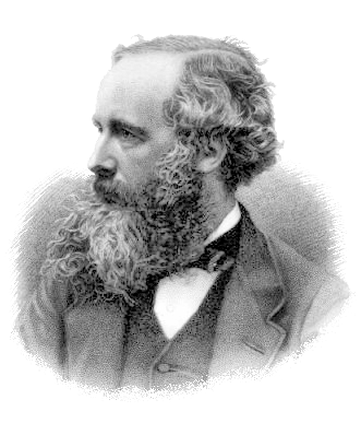
Another important figure for Cambridge was the first to derive the probability distribution that results from small balls banging together in this manner. In doing so, James Clerk Maxwell founded the field of statistical physics.

Figure: James Clerk Maxwell 1831-1879 Derived distribution of velocities of particles in an ideal gas (elastic fluid).

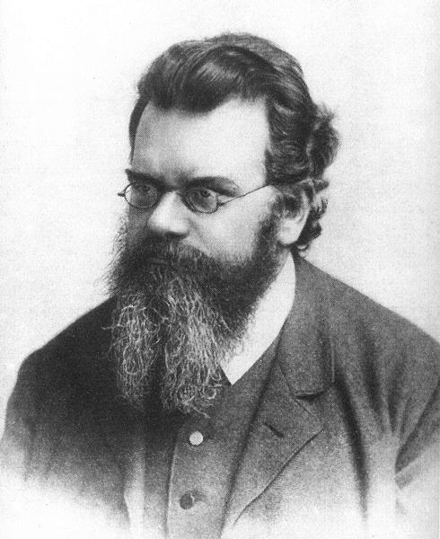
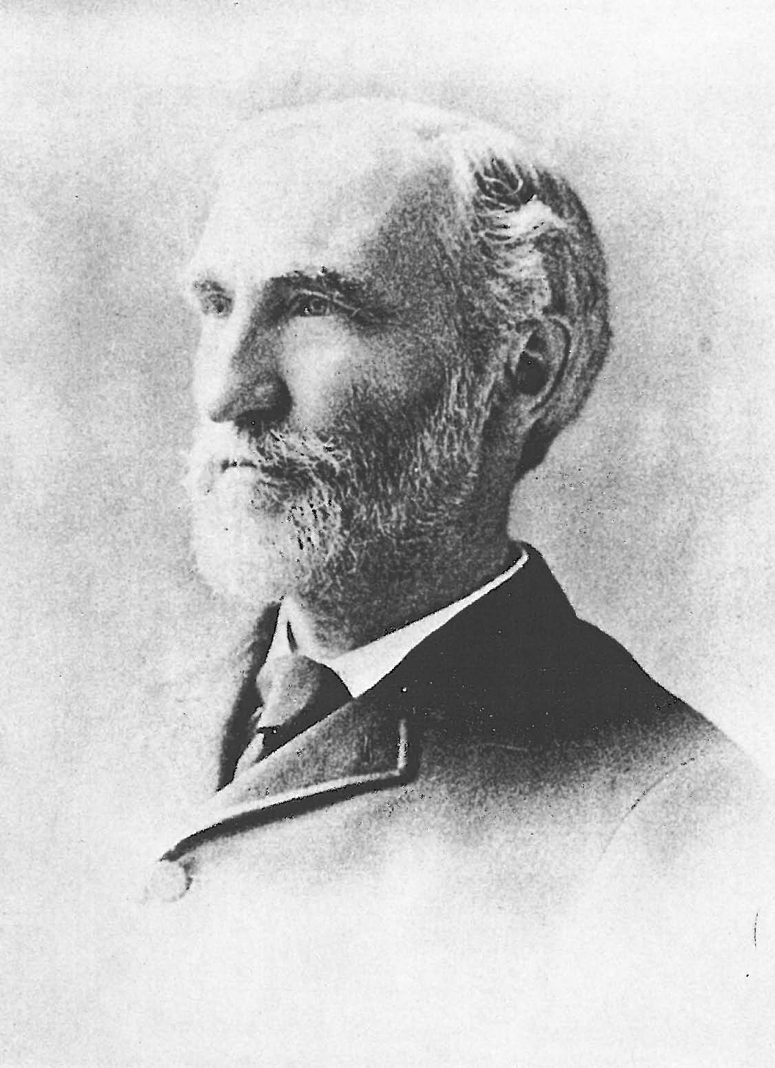
Figure: James Clerk Maxwell (1831-1879), Ludwig Boltzmann (1844-1906) Josiah Willard Gibbs (1839-1903)

Many of the ideas of early statistical physicists were rejected by a cadre of physicists who didn’t believe in the notion of a molecule. The stress of trying to have his ideas established caused Boltzmann to commit suicide in 1906, only two years before the same ideas became widely accepted.

In [ ]:

import notutils as nu
nu.display_google_book(id='Vuk5AQAAMAAJ', page='PA373')

Figure: Boltzmann’s paper Boltzmann (n.d.) which introduced the relationship between entropy and probability. A translation with notes is available in Sharp and Matschinsky (2015).

The important point about the uncertainty being represented here is that it is not genuine stochasticity, it is a lack of knowledge about the system. The techniques proposed by Maxwell, Boltzmann and Gibbs allow us to exactly represent the state of the system through a set of parameters that represent the sufficient statistics of the physical system. We know these values as the volume, temperature, and pressure. The challenge for us, when approximating the physical world with the techniques we will use is that we will have to sit somewhere between the deterministic and purely stochastic worlds that these different scientists described.

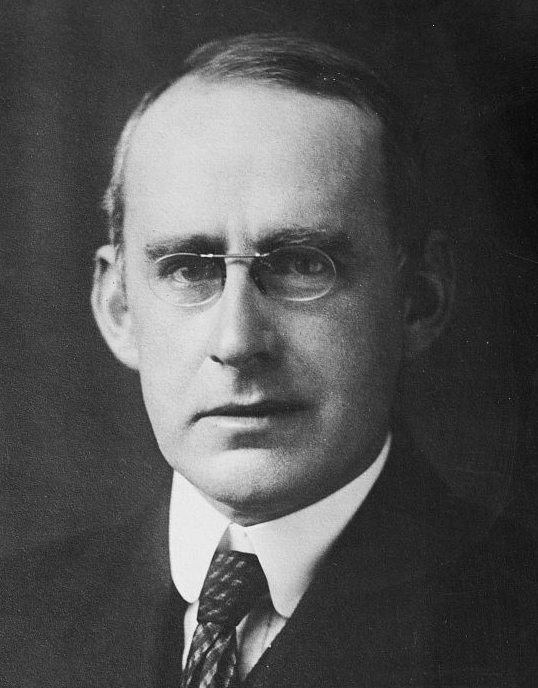
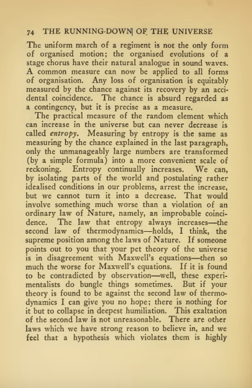
One ongoing characteristic of people who study probability and uncertainty is the confidence with which they hold opinions about it. Another leader of the Cavendish laboratory expressed his support of the second law of thermodynamics (which can be proven through the work of Gibbs/Boltzmann) with an emphatic statement at the beginning of his book.

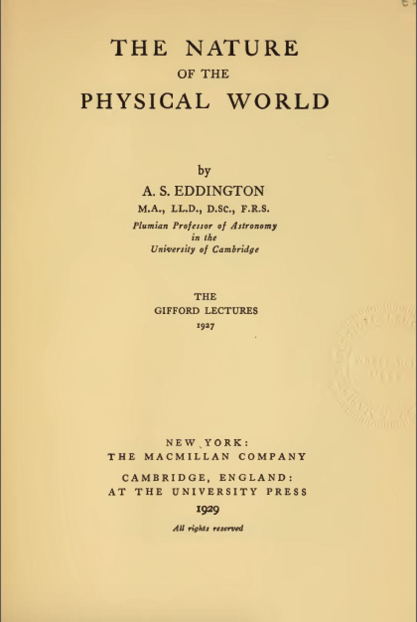
Figure: Eddington’s book on the Nature of the Physical World (Eddington, 1929)

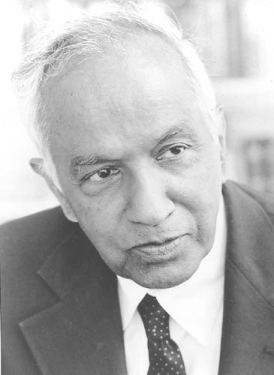
The same Eddington is also famous for dismissing the ideas of a young Chandrasekhar who had come to Cambridge to study in the Cavendish lab. Chandrasekhar demonstrated the limit at which a star would collapse under its own weight to a singularity, but when he presented the work to Eddington, he was dismissive suggesting that there “must be some natural law that prevents this abomination from happening”.

Figure: Chandrasekhar (1910-1995) derived the limit at which a star collapses in on itself. Eddington’s confidence in the 2nd law may have been what drove him to dismiss Chandrasekhar’s ideas, humiliating a young scientist who would later receive a Nobel prize for the work.

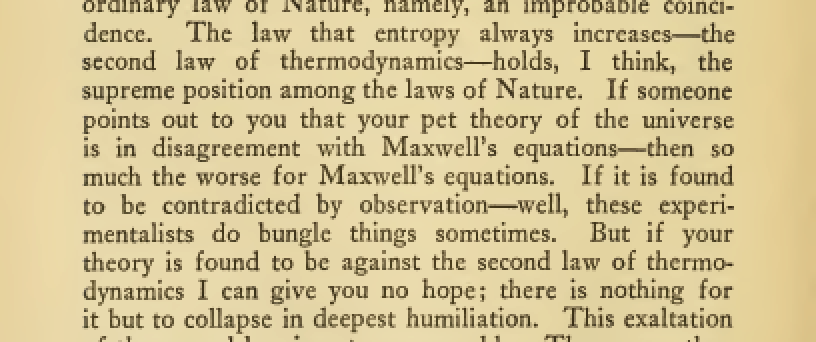
Figure: Eddington makes his feelings about the primacy of the second law clear. This primacy is perhaps because the second law can be demonstrated mathematically, building on the work of Maxwell, Gibbs and Boltzmann. Eddington (1929)

Presumably he meant that the creation of a black hole seemed to transgress the second law of thermodynamics, although later Hawking was able to show that blackholes do evaporate, but the time scales at which this evaporation occurs is many orders of magnitude slower than other processes in the universe.

Maxwell’s Demon¶

[edit]

Maxwell’s demon is a thought experiment described by James Clerk Maxwell in his book, Theory of Heat (Maxwell, 1871) on page 308.

But if we conceive a being whose faculties are so sharpened that he can follow every molecule in its course, such a being, whose attributes are still as essentially finite as our own, would be able to do what is at present impossible to us. For we have seen that the molecules in a vessel full of air at uniform temperature are moving with velocities by no means uniform, though the mean velocity of any great number of them, arbitrarily selected, is almost exactly uniform. Now let us suppose that such a vessel is divided into two portions, A and B, by a division in which there is a small hole, and that a being, who can see the individual molecules, opens and closes this hole, so as to allow only the swifter molecules to pass from A to B, and the only the slower ones to pass from B to A. He will thus, without expenditure of work, raise the temperature of B and lower that of A, in contradiction to the second law of thermodynamics.

James Clerk Maxwell in Theory of Heat (Maxwell, 1871) page 308

He goes onto say:

This is only one of the instances in which conclusions which we have draw from our experience of bodies consisting of an immense number of molecules may be found not to be applicable to the more delicate observations and experiments which we may suppose made by one who can perceive and handle the individual molecules which we deal with only in large masses

In [ ]:

import notutils as nu
nu.display_google_book(id='0p8AAAAAMAAJ', page='PA308')

Figure: Maxwell’s demon was designed to highlight the statistical nature of the second law of thermodynamics.

Entropy:

0.0000

Figure: Maxwell’s Demon. The demon decides balls are either cold (blue) or hot (red) according to their velocity. Balls are allowed to pass the green membrane from right to left only if they are cold, and from left to right, only if they are hot.

Maxwell’s demon allows us to connect thermodynamics with information theory (see e.g. Hosoya et al. (2015);Hosoya et al. (2011);Bub (2001);Brillouin (1951);Szilard (1929)). The connection arises due to a fundamental connection between information erasure and energy consumption Landauer (1961).

Alemi and Fischer (2019)

Information Theory and Thermodynamics¶

[edit]

Information theory provides a mathematical framework for quantifying information. Many of information theory’s core concepts parallel those found in thermodynamics. The theory was developed by Claude Shannon who spoke extensively to MIT’s Norbert Wiener at while it was in development (Conway and Siegelman, 2005). Wiener’s own ideas about information were inspired by Willard Gibbs, one of the pioneers of the mathematical understanding of free energy and entropy. Deep connections between physical systems and information processing have connected information and energy from the start.

Entropy¶

Shannon’s entropy measures the uncertainty or unpredictability of information content. This mathematical formulation is inspired by thermodynamic entropy, which describes the dispersal of energy in physical systems. Both concepts quantify the number of possible states and their probabilities.

Figure: Maxwell’s demon thought experiment illustrates the relationship between information and thermodynamics.

In thermodynamics, free energy represents the energy available to do work. A system naturally evolves to minimize its free energy, finding equilibrium between total energy and entropy. Free energy principles are also pervasive in variational methods in machine learning. They emerge from Bayesian approaches to learning and have been heavily promoted by e.g. Karl Friston as a model for the brain.

The relationship between entropy and Free Energy can be explored through the Legendre transform. This is most easily reviewed if we restrict ourselves to distributions in the exponential family.

Exponential Family¶

The exponential family has the form

$\rho(Z) = h(Z) \exp\left(\boldsymbol{\theta}^\top T(Z) + A(\boldsymbol{\theta})\right)$ where

$h(Z)$ is the base measure,

$\boldsymbol{\theta}$ is the natural parameters,

$T(Z)$ is the sufficient statistics and

$A(\boldsymbol{\theta})$ is the log partition function. Its entropy can be computed as

$S(Z) = A(\boldsymbol{\theta}) - \boldsymbol{\theta}^\top \nabla_\boldsymbol{\theta}A(\boldsymbol{\theta}) - E_{\rho(Z)}\left[\log h(Z)\right],$ where

$E_{\rho(Z)}[\cdot]$ is the expectation under the distribution

$\rho(Z)$ .

Available Energy¶

Work through Measurement¶

In machine learning and Bayesian inference, the Markov blanket is the set of variables that are conditionally independent of the variable of interest given the other variables. To introduce this idea into our information system, we first split the system into two parts, the variables, $X$ , and the memory $M$ .

The variables are the portion of the system that is stochastically evolving over time. The memory is a low entropy partition of the system that will give us knowledge about this evolution.

We can now write the joint entropy of the system in terms of the mutual information between the variables and the memory.

$S(Z) = S(X,M) = S(X|M) + S(M) = S(X) - I(X;M) + S(M).$ This gives us the first hint at the connection between information and energy.

If $M$ is viewed as a measurement then the change in entropy of the system before and after measurement is given by $S(X|M) - S(X)$ wehich is given by $-I(X;M)$ . This is implies that measurement increases the amount of available energy we obtain from the system (Parrondo et al., 2015).

The difference in available energy is given by

$\Delta A = A(X) - A(Z|M) = I(X;M),$ where we note that the resulting system is no longer in thermodynamic equilibrium due to the low entropy of the memory.

The Animal Game¶

[edit]

The Entropy Game is a framework for understanding efficient uncertainty reduction. To start think of finding the optimal strategy for identifying an unknown entity by asking the minimum number of yes/no questions.

The 20 Questions Paradigm¶

In the game of 20 Questions player one (Alice) thinks of an object, player two (Bob) must identify it by asking at most 20 yes/no questions. The optimal strategy is to divide the possibility space in half with each question. The binary search approach ensures maximum information gain with each inquiry and can access $2^20$ or about a million different objects.

Figure: The optimal strategy in the Entropy Game resembles a binary search, dividing the search space in half with each question.

Entropy Reduction and Decisions¶

From an information-theoretic perspective, decisions can be taken in a way that efficiently reduces entropy - our the uncertainty about the state of the world. Each observation or action an intelligent agent takes should maximize expected information gain, optimally reducing uncertainty given available resources.

The entropy before the question is $S(X)$ . The entropy after the question is $S(X|M)$ . The information gain is the difference between the two, $I(X;M) = S(X) - S(X|M)$ . Optimal decision making systems maximize this information gain per unit cost.

Thermodynamic Parallels¶

The entropy game connects decision-making to thermodynamics.

This perspective suggests a profound connection: intelligence might be understood as a special case of systems that efficiently extract, process, and utilize free energy from their environments, with thermodynamic principles setting fundamental constraints on what’s possible.

Information Engines: Intelligence as an Energy-Efficiency¶

[edit]

The entropy game shows some parallels between thermodynamics and measurement. This allows us to imagine information engines, simple systems that convert information to energy. This is our first simple model of intelligence.

Measurement as a Thermodynamic Process: Information-Modified Second Law¶

The second law of thermodynamics was generalised to include the effect of measurement by Sagawa and Ueda (Sagawa and Ueda, 2008). They showed that the maximum extractable work from a system can be increased by $k_BTI(X;M)$ where $k_B$ is Boltzmann’s constant, $T$ is temperature and $I(X;M)$ is the information gained by making a measurement, $M$ ,

$I(X;M) = \sum_{x,m} \rho(x,m) \log \frac{\rho(x,m)}{\rho(x)\rho(m)},$ where

$\rho(x,m)$ is the joint probability of the system and measurement (see e.g. eq 14 in Sagawa and Ueda (2008)). This can be written as

$W_\text{ext} \leq - \Delta\mathcal{F} + k_BTI(X;M),$ where

$W_\text{ext}$ is the extractable work and it is upper bounded by the negative change in free energy,

$\Delta \mathcal{F}$ , plus the energy gained from measurement,

$k_BTI(X;M)$ . This is the information-modified second law.

The measurements can be seen as a thermodynamic process. In theory measurement, like computation is reversible. But in practice the process of measurement is likely to erode the free energy somewhat, but as long as the energy gained from information, $kTI(X;M)$ is greater than that spent in measurement the pricess can be thermodynamically efficient.

The modified second law shows that the maximum additional extractable work is proportional to the information gained. So information acquisition creates extractable work potential. Thermodynamic consistency is maintained by properly accounting for information-entropy relationships.

Efficacy of Feedback Control¶

Sagawa and Ueda extended this relationship to provide a generalised Jarzynski equality for feedback processes (Sagawa and Ueda, 2010). The Jarzynski equality is an imporant result from nonequilibrium thermodynamics that relates the average work done across an ensemble to the free energy difference between initial and final states (Jarzynski, 1997),

$\left\langle \exp\left(-\frac{W}{k_B T}\right) \right\rangle = \exp\left(-\frac{\Delta\mathcal{F}}{k_BT}\right),$ where

$\langle W \rangle$ is the average work done across an ensemble of trajectories,

$\Delta\mathcal{F}$ is the change in free energy,

$k_B$ is Boltzmann’s constant, and

$\Delta S$ is the change in entropy. Sagawa and Ueda extended this equality to to include information gain from measurement (Sagawa and Ueda, 2010),

$\left\langle \exp\left(-\frac{W}{k_B T}\right) \exp\left(\frac{\Delta\mathcal{F}}{k_BT}\right) \exp\left(-\mathcal{I}(X;M)\right)\right\rangle = 1,$ where

$\mathcal{I}(X;M) = \log \frac{\rho(X|M)}{\rho(X)}$ is the information gain from measurement, and the mutual information is recovered

$I(X;M) = \left\langle \mathcal{I}(X;M) \right\rangle$ as the average information gain.

Sagawa and Ueda introduce an efficacy term that captures the effect of feedback on the system they note in the presence of feedback,

$\left\langle \exp\left(-\frac{W}{k_B T}\right) \exp\left(\frac{\Delta\mathcal{F}}{k_BT}\right)\right\rangle = \gamma,$ where

$\gamma$ is the efficacy.

Channel Coding Perspective on Memory¶

When viewing $M$ as an information channel between past and future states, Shannon’s channel coding theorems apply (Shannon, 1948). The channel capacity $C$ represents the maximum rate of reliable information transmission [ C = _{(M)} I(X_1;M) ] and for a memory of $n$ bits we have [ C n, ] as the mutual information is upper bounded by the entropy of $\rho(M)$ which is at most $n$ bits.

This relationship seems to align with Ashby’s Law of Requisite Variety (pg 229 Ashby (1952)), which states that a control system must have at least as much ‘variety’ as the system it aims to control. In the context of memory systems, this means that to maintain temporal correlations effectively, the memory’s state space must be at least as large as the information content it needs to preserve. This provides a lower bound on the necessary memory capacity that complements the bound we get from Shannon for channel capacity.

This helps determine the required memory size for maintaining temporal correlations, optimal coding strategies, and fundamental limits on temporal correlation preservation.

Decomposition into Past and Future¶

Model Approximations and Thermodynamic Efficiency¶

Intelligent systems must balance measurement against energy efficiency and time requirements. A perfect model of the world would require infinite computational resources and speed, so approximations are necessary. This leads to uncertainties. Thermodynamics might be thought of as the physics of uncertainty: at equilibrium thermodynamic systems find thermodynamic states that minimize free energy, equivalent to maximising entropy.

Markov Blanket¶

To introduce some structure to the model assumption. We split $X$ into $X_0$ and $X_1$ . $X_0$ is past and present of the system, $X_1$ is future The conditional mutual information $I(X_0;X_1|M)$ which is zero if $X_1$ and $X_0$ are independent conditioned on $M$ .

At What Scales Does this Apply?¶

The equipartition theorem tells us that at equilibrium the average energy is $kT/2$ per degree of freedom. This means that for systems that operate at “human scale” the energy involved is many orders of magnitude larger than the amount of information we can store in memory. For a car engine producing 70 kW of power at 370 Kelvin, this implies

$\frac{2 \times 70,000}{370 \times k_B} = \frac{2 \times 70,000}{370\times 1.380649×10^{−23}} = 2.74 × 10^{25}$ degrees of freedom per second. If we make a conservative assumption of one bit per degree of freedom, then the mutual information we would require in one second for comparative energy production would be around 3400 zettabytes, implying a memory bandwidth of around 3,400 zettabytes per second. In 2025 the estimate of all the data in the world stands at 149 zettabytes.

Small-Scale Biochemical Systems and Information Processing¶

While macroscopic systems operate in regimes where traditional thermodynamics dominates, microscopic biological systems operate at scales where information and thermal fluctuations become critically important. Here we examine how the framework applies to molecular machines and processes that have evolved to operate efficiently at these scales.

Molecular machines like ATP synthase, kinesin motors, and the photosynthetic apparatus can be viewed as sophisticated information engines that convert energy while processing information about their environment. These systems have evolved to exploit thermal fluctuations rather than fight against them, using information processing to extract useful work.

ATP Synthase: Nature’s Rotary Engine¶

ATP synthase functions as a rotary molecular motor that synthesizes ATP from ADP and inorganic phosphate using a proton gradient. The system uses the proton gradient as both an energy source and an information source about the cell’s energetic state and exploits Brownian motion through a ratchet mechanism. It converts information about proton locations into mechanical rotation and ultimately chemical energy with approximately 3-4 protons required per ATP.

In [ ]:

from IPython.lib.display import YouTubeVideo
YouTubeVideo('kXpzp4RDGJI')

Estimates suggest that one synapse firing may require $10^4$ ATP molecules, so around $4 \times 10^4$ protons. If we take the human brain as containing around $10^{14}$ synapses, and if we suggest each synapse only fires about once every five seconds, we would require approximately $10^{18}$ protons per second to power the synapses in our brain. With each proton having six degrees of freedom. Under these rough calculations the memory capacity distributed across the ATP Synthase in our brain must be of order $6 \times 10^{18}$ bits per second or 750 petabytes of information per second. Of course this memory capacity would be devolved across the billions of neurons within hundreds or thousands of mitochondria that each can contain thousands of ATP synthase molecules. By composition of extremely small systems we can see it’s possible to improve efficiencies in ways that seem very impractical for a car engine.

Quick note to clarify, here we’re referring to the information requirements to make our brain more energy efficient in its information processing rather than the information processing capabilities of the neurons themselves!

Jaynes’ World¶

[edit]

Jaynes’ World is a zero-player game that implements a version of the entropy game. The dynamical system is defined by a distribution, $\rho(Z)$ , over a state space $Z$ . The state space is partitioned into observable variables $X$ and memory variables $M$ . The memory variables are considered to be in an information resevoir, a thermodynamic system that maintains information in an ordered state (see e.g. Barato and Seifert (2014)). The entropy of the whole system is bounded below by 0 and above by $N$ . So the entropy forms a compact manifold with respect to its parameters.

Unlike the animal game, where decisions are made by reducing entropy at each step, our system evovles mathematically by maximising the instantaneous entropy production. Conceptually we can think of this as ascending the gradient of the entropy, $S(Z)$ .

In the animal game the questioner starts with maximum uncertainty and targets minimal uncertainty. Jaynes’ world starts with minimal uncertainty and aims for maximum uncertainty.

We can phrase this as a thought experiment. Imagine you are in the game, at a given turn. You want to see where the game came from, so you look back across turns. The direction the game came from is now the direction of steepest descent. Regardless of where the game actually started it looks like it started at a minimal entropy configuration that we call the origin. Similarly, wherever the game is actually stopped there will nevertheless appear to be an end point we call end that will be a configuration of maximal entropy, $N$ .

This speculation allows us to impose the functional form of our proability distribution. As Jaynes has shown (Jaynes, 1957), the stationary points of a free-form optimisation (minimum or maximum) will place the distribution in the, $\rho(Z)$ in the exponential family,

$\rho(Z) = h(Z) \exp(\boldsymbol{\theta}^\top T(Z) - A(\boldsymbol{\theta})),$ where

$h(Z)$ is the base measure,

$T(Z)$ are sufficient statistics,

$A(\boldsymbol{\theta})$ is the log-partition function,

$\boldsymbol{\theta}$ are the natural parameters of the distribution.}

This constraint to the exponential family is highly convenient as we will rely on it heavily for the dynamics of the game. In particular, by focussing on the natural parameters we find that we are optimising within an information geometry (Amari, 2016). In exponential family distributions, the entropy gradient is given by,

$\nabla_{\boldsymbol{\theta}}S(Z) = \mathbf{g} = \nabla^2_\boldsymbol{\theta} A(\boldsymbol{\theta}(M))$ And the Fisher information matrix,

$G(\boldsymbol{\theta})$ , is also the Hessian of the manifold,

$G(\boldsymbol{\theta}) = \nabla^2_{\boldsymbol{\theta}} A(\boldsymbol{\theta}) = \text{Cov}[T(Z)].$ Traditionally, when optimising on an information geometry we take natural gradient steps, equivalen to a Newton minimisation step,

$\Delta \boldsymbol{\theta} = - G(\boldsymbol{\theta})^{-1} \mathbf{g},$ but this is not the direction that gives the instantaneious maximisation of the entropy production, instead our gradient step is given by

$\Delta \boldsymbol{\theta} = \eta \mathbf{g},$ where

$\eta$ is a ‘learning rate’.

Markovian Decomposition¶

Now $X$ is further divided into past/present $X_0$ and future $X_1$ . The entropy can be decomposed into a Markovian component, where $X_0$ and $X_1$ are conditionally independent given $M$ and a non-Markovian component. The conditional mutual information is

$I(X_0; X_1 | M) = \sum_{x_0,x_1,m} p(x_0,x_1,m) \log \frac{p(x_0,x_1|m)}{p(x_0|m)p(x_1|m)},$ which measures the remaining dependency between past and future given the memory state. This leads to a key insight about memory capacity: effective information reservoirs must minimize this conditional mutual information while maintaining minimal entropy.

When $I(X_0; X_1 | M) = 0$ , the system becomes perfectly Markovian - the memory variables capture all dependencies between past and future. However, achieving this perfect Markovianity while maintaining minimal entropy in $M$ will create a fundamental tension that drives an uncertainty principle.

System Evolution¶

We are now in a position to summarise the start state and the end state of our system, as well as to speculate on the nature of the transition between the two states.

Start State¶

The origin configuration is a low entropy state, with value near the lower bound of 0. The information is highly structured, by definition we place all variables in $M$ , the information resevoir at this time. The uncertainty principle is present to handle the competeing needs of precision in parameters (giving us the near-singular form for $\boldsymbol{\theta}(M)$ , and capacity in the information channel that $M$ provides (the capacity $c(\boldsymbol{\theta})$ is upper bounded by $S(M)$ .

End State¶

The end configuration is a high entropy state, near the upper bound. Both the minimal entropy and maximal entropy states are revealed by Ed Jaynes’ variational minimisation approach and are in the exponential family. In many cases a version of Zeno’s paradox will arise where the system asymtotes to the final state, taking smaller steps at each time. At this point the system is at equilibrium.

Histogram Game¶

[edit]

To illustrate the concept of the Jaynes’ world entropy game we’ll run a simple example using a four bin histogram. The entropy of a four bin histogram can be computed as,

$S(p) = - \sum_{i=1}^4 p_i \log_2 p_i.$

In [ ]:

import numpy as np

First we write some helper code to plot the histogram and compute its entropy.

In [ ]:

import matplotlib.pyplot as plt
import mlai.plot as plot

In [ ]:

def plot_histogram(ax, p, max_height=None):
    heights = p
    if max_height is None:
        max_height = 1.25*heights.max()
    
    # Safe entropy calculation that handles zeros
    nonzero_p = p[p > 0]  # Filter out zeros
    S = - (nonzero_p*np.log2(nonzero_p)).sum()

    # Define bin edges
    bins = [1, 2, 3, 4, 5]  # Bin edges

    # Create the histogram
    if ax is None:
        fig, ax = plt.subplots(figsize=(6, 4))  # Adjust figure size 
    ax.hist(bins[:-1], bins=bins, weights=heights, align='left', rwidth=0.8, edgecolor='black') # Use weights for probabilities


    # Customize the plot for better slide presentation
    ax.set_xlabel("Bin")
    ax.set_ylabel("Probability")
    ax.set_title(f"Four Bin Histogram (Entropy {S:.3f})")
    ax.set_xticks(bins[:-1]) # Show correct x ticks
    ax.set_ylim(0,max_height) # Set y limit for visual appeal

We can compute the entropy of any given histogram.

In [ ]:

# Define probabilities
p = np.zeros(4)
p[0] = 4/13
p[1] = 3/13
p[2] = 3.7/13
p[3] = 1 - p.sum()

# Safe entropy calculation
nonzero_p = p[p > 0]  # Filter out zeros
entropy = - (nonzero_p*np.log2(nonzero_p)).sum()
print(f"The entropy of the histogram is {entropy:.3f}.")

In [ ]:

import matplotlib.pyplot as plt
import mlai.plot as plot
import mlai

In [ ]:

fig, ax = plt.subplots(figsize=plot.big_wide_figsize)
fig.tight_layout()
plot_histogram(ax, p)
ax.set_title(f"Four Bin Histogram (Entropy {entropy:.3f})")
mlai.write_figure(filename='four-bin-histogram.svg', 
                  directory = './information-game')

Figure: The entropy of a four bin histogram.

We can play the entropy game by starting with a histogram with all the probability mass in the first bin and then ascending the gradient of the entropy function. To do this we represent the histogram parameters as a vector of length 4, $\mathbf{ w}{\lambda} = [\lambda_1, \lambda_2, \lambda_3, \lambda_4]$ and define the histogram probabilities to be $p_i = \lambda_i^2 / \sum_{j=1}^4 \lambda_j^2$ .

In [ ]:

import numpy as np

In [ ]:

# Define the entropy function 
def entropy(lambdas):
    p = lambdas**2/(lambdas**2).sum()
    
    # Safe entropy calculation
    nonzero_p = p[p > 0]
    nonzero_lambdas = lambdas[p > 0]
    return np.log2(np.sum(lambdas**2))-np.sum(nonzero_p * np.log2(nonzero_lambdas**2))

# Define the gradient of the entropy function
def entropy_gradient(lambdas):
    denominator = np.sum(lambdas**2)
    p = lambdas**2/denominator
    
    # Safe log calculation
    log_terms = np.zeros_like(lambdas)
    nonzero_idx = lambdas != 0
    log_terms[nonzero_idx] = np.log2(np.abs(lambdas[nonzero_idx]))
    
    p_times_lambda_entropy = -2*log_terms/denominator
    const = (p*p_times_lambda_entropy).sum()
    gradient = 2*lambdas*(p_times_lambda_entropy - const)
    return gradient

# Numerical gradient check
def numerical_gradient(func, lambdas, h=1e-5):
    numerical_grad = np.zeros_like(lambdas)
    for i in range(len(lambdas)):
        temp_lambda_plus = lambdas.copy()
        temp_lambda_plus[i] += h
        temp_lambda_minus = lambdas.copy()
        temp_lambda_minus[i] -= h
        numerical_grad[i] = (func(temp_lambda_plus) - func(temp_lambda_minus)) / (2 * h)
    return numerical_grad

We can then ascend the gradeint of the entropy function, starting at a parameter setting where the mass is placed in the first bin, we take $\lambda_2 = \lambda_3 = \lambda_4 = 0.01$ and $\lambda_1 = 100$ .

First to check our code we compare our numerical and analytic gradients.

In [ ]:

import numpy as np

In [ ]:

# Initial parameters (lambda)
initial_lambdas = np.array([100, 0.01, 0.01, 0.01])

# Gradient check
numerical_grad = numerical_gradient(entropy, initial_lambdas)
analytical_grad = entropy_gradient(initial_lambdas)
print("Numerical Gradient:", numerical_grad)
print("Analytical Gradient:", analytical_grad)
print("Gradient Difference:", np.linalg.norm(numerical_grad - analytical_grad))  # Check if close to zero

Now we can run the steepest ascent algorithm.

In [ ]:

import numpy as np

In [ ]:

# Steepest ascent algorithm
lambdas = initial_lambdas.copy()

learning_rate = 1
turns = 15000
entropy_values = []
lambdas_history = []

for _ in range(turns):
    grad = entropy_gradient(lambdas)
    lambdas += learning_rate * grad # update lambda for steepest ascent
    entropy_values.append(entropy(lambdas))
    lambdas_history.append(lambdas.copy())

We can plot the histogram at a set of chosen turn numbers to see the progress of the algorithm.

In [ ]:

import matplotlib.pyplot as plt
import mlai.plot as plot
import mlai

In [ ]:

fig, ax = plt.subplots(figsize=plot.big_wide_figsize)
plot_at = [0, 100, 1000, 2500, 5000, 7500, 10000, 12500, turns-1]
for i, iter in enumerate(plot_at):
    plot_histogram(ax, lambdas_history[i]**2/(lambdas_history[i]**2).sum(), 1)
    # write the figure,
    mlai.write_figure(filename=f'four-bin-histogram-turn-{i:02d}.svg', 
                      directory = './information-game')

In [ ]:

import notutils as nu
from ipywidgets import IntSlider

In [ ]:

nu.display_plots('two_point_sample{sample:0>3}.svg', 
                            './information-game', 
                            sample=IntSlider(5, 5, 5, 1))

¶

Figure: Intermediate stages of the histogram entropy game. After 0, 1000, 5000, 10000 and 15000 iterations.

And we can also plot the changing entropy as a function of the number of game turns.

In [ ]:

fig, ax = plt.subplots(figsize=plot.big_wide_figsize)
ax.plot(range(turns), entropy_values)
ax.set_xlabel("turns")
ax.set_ylabel("entropy")
ax.set_title("Entropy vs. turns (Steepest Ascent)")
mlai.write_figure(filename='four-bin-histogram-entropy-vs-turns.svg', 
                  directory = './information-game')

Figure: Four bin histogram entropy game. The plot shows the increasing entropy against the number of turns across 15000 iterations of gradient ascent.

Note that the entropy starts at a saddle point, increaseases rapidly, and the levels off towards the maximum entropy, with the gradient decreasing slowly in the manner of Zeno’s paradox.

Two-Bin Histogram Example¶

[edit]

The simplest possible example of Jaynes’ World is a two-bin histogram with probabilities $p$ and $1-p$ . This minimal system allows us to visualize the entire entropy landscape.

The natural parameter is the log odds, $\theta = \log\frac{p}{1-p}$ , and the update given by the entropy gradient is

$\Delta \theta_{\text{steepest}} = \eta \frac{\text{d}S}{\text{d}\theta} = \eta p(1-p)(\log(1-p) - \log p).$ The Fisher information is

$G(\theta) = p(1-p)$ This creates a dynamic where as

$p$ approaches either 0 or 1 (minimal entropy states), the Fisher information approaches zero, creating a critical slowing” effect. This critical slowing is what leads to the formation of information resevoirs. Note also that in the natural gradient the updated is given by multiplying the gradient by the inverse Fisher information, which would lead to a more efficient update of the form,

$\Delta \theta_{\text{natural}} = \eta(\log(1-p) - \log p),$ however, it is precisely this efficiency that we want our game to avoid, because it is the inefficient behaviour in the reagion of saddle points that leads to critical slowing and the emergence of information resevoirs.

In [ ]:

import numpy as np

In [ ]:

# Python code for gradients
p_values = np.linspace(0.000001, 0.999999, 10000)
theta_values = np.log(p_values/(1-p_values))
entropy = -p_values * np.log(p_values) - (1-p_values) * np.log(1-p_values)
fisher_info = p_values * (1-p_values)
gradient = fisher_info * (np.log(1-p_values) - np.log(p_values))

In [ ]:

import matplotlib.pyplot as plt
import mlai.plot as plot
import mlai

In [ ]:

fig, (ax1, ax2) = plt.subplots(1, 2, figsize=plot.big_wide_figsize)

ax1.plot(theta_values, entropy)
ax1.set_xlabel('$\\theta$')
ax1.set_ylabel('Entropy $S(p)$')
ax1.set_title('Entropy Landscape')

ax2.plot(theta_values, gradient)
ax2.set_xlabel('$\\theta$')
ax2.set_ylabel('$\\nabla_\\theta S(p)$')
ax2.set_title('Entropy Gradient vs. Position')

mlai.write_figure(filename='two-bin-histogram-entropy-gradients.svg', 
                  directory = './information-game')

Figure: Entropy gradients of the two bin histogram agains position.

This simple example reveals the entropy extrema at $p = 0$ , $p = 0.5$ , and $p = 1$ . At minimal entropy ( $p \approx 0$ or $p \approx 1$ ), the gradient approaches zero, creating natural information reservoirs. The dynamics slow dramatically near these points - these are the areas of critical slowing that create information reservoirs.

Four-Bin Saddle Point Example¶

[edit]

To illustrate saddle points and information reservoirs, we need at least a 4-bin system. This creates a 3-dimensional parameter space where we can observe genuine saddle points.

Consider a 4-bin system parameterized by natural parameters $\theta_1$ , $\theta_2$ , and $\theta_3$ (with one constraint). A saddle point occurs where the gradient $\nabla_\theta S = 0$ , but the Hessian has mixed eigenvalues - some positive, some negative.

At these points, the Fisher information matrix $G(\theta)$ eigendecomposition reveals.

Fast modes: large positive eigenvalues → rapid evolution
Slow modes: small positive eigenvalues → gradual evolution
Critical modes: near-zero eigenvalues → information reservoirs

The eigenvectors of $G(\theta)$ at the saddle point determine which parameter combinations form information reservoirs.

In [ ]:

import numpy as np

In [ ]:

# Exponential family entropy with saddle point
def exponential_family_entropy(theta1, theta2, theta3=None):
    """
    Compute entropy of a 4-bin exponential family distribution
    parameterized by natural parameters theta1, theta2, theta3
    (with the constraint that probabilities sum to 1)
    """
    # If theta3 is not provided, we'll use a function of theta1 and theta2
    if theta3 is None:
        theta3 = -0.5 * (theta1 + theta2)
    
    # Compute the log-partition function (normalization constant)
    theta4 = -(theta1 + theta2 + theta3)  # Constraint
    log_Z = np.log(np.exp(theta1) + np.exp(theta2) + np.exp(theta3) + np.exp(theta4))
    
    # Compute probabilities
    p1 = np.exp(theta1 - log_Z)
    p2 = np.exp(theta2 - log_Z)
    p3 = np.exp(theta3 - log_Z)
    p4 = np.exp(theta4 - log_Z)
    
    # Compute entropy: -sum(p_i * log(p_i))
    entropy = -np.sum(
        np.array([p1, p2, p3, p4]) * 
        np.log(np.array([p1, p2, p3, p4])), 
        axis=0, where=np.array([p1, p2, p3, p4])>0
    )
    
    return entropy

def entropy_gradient(theta1, theta2, theta3=None):
    """
    Compute the gradient of the entropy with respect to theta1 and theta2
    """
    # If theta3 is not provided, we'll use a function of theta1 and theta2
    if theta3 is None:
        theta3 = -0.5 * (theta1 + theta2)
    
    # Compute the log-partition function
    theta4 = -(theta1 + theta2 + theta3)  # Constraint
    log_Z = np.log(np.exp(theta1) + np.exp(theta2) + np.exp(theta3) + np.exp(theta4))
    
    # Compute probabilities
    p1 = np.exp(theta1 - log_Z)
    p2 = np.exp(theta2 - log_Z)
    p3 = np.exp(theta3 - log_Z)
    p4 = np.exp(theta4 - log_Z)
    
    # For the gradient, we need to account for the constraint on theta3
    # When theta3 = -0.5(theta1 + theta2), we have:
    # theta4 = -(theta1 + theta2 + theta3) = -(theta1 + theta2 - 0.5(theta1 + theta2)) = -0.5(theta1 + theta2)
    
    # Gradient components with chain rule applied
    # For theta1: ∂S/∂theta1 + ∂S/∂theta3 * ∂theta3/∂theta1 + ∂S/∂theta4 * ∂theta4/∂theta1
    grad_theta1 = (p1 * (np.log(p1) + 1)) - 0.5 * (p3 * (np.log(p3) + 1)) - 0.5 * (p4 * (np.log(p4) + 1))
    
    # For theta2: ∂S/∂theta2 + ∂S/∂theta3 * ∂theta3/∂theta2 + ∂S/∂theta4 * ∂theta4/∂theta2
    grad_theta2 = (p2 * (np.log(p2) + 1)) - 0.5 * (p3 * (np.log(p3) + 1)) - 0.5 * (p4 * (np.log(p4) + 1))
    
    return grad_theta1, grad_theta2

# Create a grid of points
x = np.linspace(-2, 2, 100)
y = np.linspace(-2, 2, 100)
X, Y = np.meshgrid(x, y)

# Compute entropy and its gradient at each point
Z = exponential_family_entropy(X, Y)
dX, dY = entropy_gradient(X, Y)

# Normalize gradient vectors for better visualization
norm = np.sqrt(dX**2 + dY**2)
# Avoid division by zero
norm = np.where(norm < 1e-10, 1e-10, norm)
dX_norm = dX / norm
dY_norm = dY / norm

# A few gradient vectors for visualization
stride = 10

In [ ]:

import matplotlib.pyplot as plt
import mlai.plot as plot
import mlai

In [ ]:

fig = plt.figure(figsize=plot.big_wide_figsize)

# Create contour lines only (no filled contours)
contours = plt.contour(X, Y, Z, levels=15, colors='black', linewidths=0.8)
plt.clabel(contours, inline=True, fontsize=8, fmt='%.2f')

# Add gradient vectors (normalized for direction, but scaled by magnitude for visibility)
# Note: We're using the negative of the gradient to point in direction of increasing entropy
plt.quiver(X[::stride, ::stride], Y[::stride, ::stride], 
           -dX_norm[::stride, ::stride], -dY_norm[::stride, ::stride], 
           color='r', scale=30, width=0.003, scale_units='width')

# Add labels and title
plt.xlabel('$\\theta_1$')
plt.ylabel('$\\theta_2$')
plt.title('Entropy Contours with Gradient Field')

# Mark the saddle point (approximately at origin for this system)
plt.scatter([0], [0], color='yellow', s=100, marker='*', 
            edgecolor='black', zorder=10, label='Saddle Point')
plt.legend()

mlai.write_figure(filename='simplified-saddle-point-example.svg', 
                  directory = './information-game')

Figure: Visualisation of a saddle point projected down to two dimensions.

The animation of system evolution would show initial rapid movement along high-eigenvalue directions, progressive slowing in directions with low eigenvalues and formation of information reservoirs in the critically slowed directions. Parameter-capacity uncertainty emerges naturally at the saddle point.

Saddle Points¶

[edit]

Saddle points represent critical transitions in the game’s evolution where the gradient $\nabla_{\boldsymbol{\theta}}S \approx 0$ but the game is not at a maximum or minimum. At these points.

The Fisher information matrix $G(\boldsymbol{\theta})$ has eigenvalues with significantly different magnitudes
Some eigenvalues approach zero, creating “critically slowed” directions in parameter space
Other eigenvalues remain large, allowing rapid evolution in certain directions

This creates a natural separation between “memory” variables (associated with near-zero eigenvalues) and “processing” variables (associated with large eigenvalues). The game’s behavior becomes highly non-isotropic in parameter space.

At saddle points, direct gradient ascent stalls, and the game must leverage the Fourier duality between parameters and capacity variables to continue entropy production. The duality relationship

$c(M) = \mathcal{F}[\boldsymbol{\theta}(M)]$ allows the game to progress by temporarily increasing uncertainty in capacity space, which creates gradients in previously flat directions of parameter space.

These saddle points often coincide with phase transitions between parameter-dominated and capacity-dominated regimes, where the game’s fundamental character changes in terms of information processing capabilities.

Saddle Point Seeking Behaviour¶

In the game’s evolution, we follow steepest ascent in parameter space to maximize entropy. Let’s contrast with the natural gradient approach that is often used in information geometry.

The steepest ascent direction in Euclidean space is given by,

$\Delta \boldsymbol{\theta}_{\text{steepest}} = \eta \nabla_{\boldsymbol{\theta}} S = \eta \mathbf{g}$ where

$\eta$ is a learning rate and

$\mathbf{g}$ is the entropy gradient.

In contrast, the natural gradient adjusts the update direction according to the Fisher information geometry,

$\Delta \boldsymbol{\theta}_{\text{natural}} = \eta G(\boldsymbol{\theta})^{-1} \nabla_{\boldsymbol{\theta}} S = \eta G(\boldsymbol{\theta})^{-1} \mathbf{g}$ where

$G(\boldsymbol{\theta})$ is the Fisher information matrix. This represents a Newton step in the natural parameter space. Often the Newton step is difficult to compute, but for exponential families and their entropies the Fisher information has a form closely related to the gradients and would be easy to leverage. The game explicitly uses steepest ascent and this leads to very different behaviour, in particular near saddle points. In this regime

Steepest ascent slows dramatically in directions where the gradient is small, leading to extremely slow progress along the critically slowed modes. This actually helps the game by preserving information in these modes while allowing continued evolution in other directions.
Natural gradient would normalize the updates by the Fisher information, potentially accelerating progress in critically slowed directions. This would destroy the natural emergence of information reservoirs that we desire.

The use of steepest ascent rather than natural gradient is deliberate in our game. It allows the Fisher information matrix’s eigenvalue structure to directly influence the temporal dynamics, creating a natural separation of timescales that preserves information in critically slowed modes while allowing rapid evolution in others.

As the game approaches a saddle point

The gradient $\nabla_{\boldsymbol{\theta}} S$ approaches zero in some directions but remains non-zero in others
The eigendecomposition of the Fisher information matrix $G(\boldsymbol{\theta}) = V \Lambda V^T$ reveals which directions are critically slowed
Update magnitudes in different directions become proportional to their corresponding eigenvalues
This creates the hierarchical timescale separation that forms the basis of our memory structure

This behavior creates a computational architecture where different variables naturally assume different functional roles based on their update dynamics, without requiring explicit design. The information geometry of the parameter space, combined with steepest ascent dynamics, self-organizes the game into memory and processing components.

Gradient Flow and Least Action Principles¶

[edit]

The steepest ascent dynamics in our system naturally connect to least action principles in physics. We can demonstrate this connection through a simple visualisation of gradient flows.

For our entropy game, we can define an information-theoretic action,

$\mathcal{A}[\gamma] = \int_0^T \left(\frac{1}{2}\dot{\boldsymbol{\theta}}^\top G(\boldsymbol{\theta}) \dot{\boldsymbol{\theta}} - S(\boldsymbol{\theta})\right) \text{d}t$ where

$\gamma$ is a path through parameter space,

$G(\boldsymbol{\theta})$ is the Fisher information matrix, and

$S(\boldsymbol{\theta})$ is the entropy. The least action principle states that the system will follow paths that extremise this action.

This is also what our steepest ascent dynamics produce: the system follows geodesics in the information geometry while maximizing entropy production. As the system evolves, it naturally creates information reservoirs in directions where the gradient is small but non-zero.

In [ ]:

import numpy as np

In [ ]:

# Create a potential energy landscape based on bivariate Gaussian entropy
def potential(x, y):
    # Interpret x as sqrt-precision parameter and y as correlation parameter
    # Constrain y to be between -1 and 1 (valid correlation)
    y_corr = np.tanh(y)
    
    # Construct precision and covariance matrices
    precision = x**2  # x is sqrt-precision
    variance = 1/precision
    covariance = y_corr * variance
    
    # Covariance matrix
    Sigma = np.array([[variance, covariance], 
                      [covariance, variance]])
    
    # Entropy of bivariate Gaussian
    det_Sigma = variance**2 * (1 - y_corr**2)
    entropy = 0.5 * np.log((2 * np.pi * np.e)**2 * det_Sigma)
    
    return entropy

# Create gradient vector field for the Gaussian entropy
def gradient(x, y):
    # Small delta for numerical gradient
    delta = 1e-6
    
    # Compute numerical gradient
    dx = (potential(x + delta, y) - potential(x - delta, y)) / (2 * delta)
    dy = (potential(x, y + delta) - potential(x, y - delta)) / (2 * delta)
    
    return dx, dy

# Simulate and plot a particle path following gradient
def simulate_path(start_x, start_y, steps=100000, dt=0.00001):
    path_x, path_y = [start_x], [start_y]
    x, y = start_x, start_y
    for _ in range(steps):
        dx_val, dy_val = gradient(x, y)
        x += dx_val * dt
        y += dy_val * dt
        path_x.append(x)
        path_y.append(y)
    return path_x, path_y

In [ ]:

# Visualizing gradient flow and least action path

# Create grid
x = np.linspace(-3, 4, 100)
y = np.linspace(-3, 4, 100)
X, Y = np.meshgrid(x, y)
Z = potential(X, Y)

# Calculate gradient field
dx, dy = gradient(X, Y)
magnitude = np.sqrt(dx**2 + dy**2)
path_x, path_y = simulate_path(2, 3)

In [ ]:

import matplotlib.pyplot as plt
import mlai.plot as plot
import mlai
from matplotlib.colors import LogNorm

In [ ]:

# Create the figure
fig, ax = plt.subplots(figsize=(10, 8))

# Plot potential as contour lines only (not filled)
contour = ax.contour(X, Y, Z, levels=15, colors='black', alpha=0.7, linewidths=0.8)
ax.clabel(contour, inline=True, fontsize=8)  # Add labels to contour lines

# Plot gradient field
stride = 5
ax.quiver(X[::stride, ::stride], Y[::stride, ::stride], 
          dx[::stride, ::stride]/magnitude[::stride, ::stride], 
          dy[::stride, ::stride]/magnitude[::stride, ::stride],
          magnitude[::stride, ::stride],
          cmap='autumn', scale=25, width=0.002)

# Plot path
ax.plot(path_x, path_y, 'r-', linewidth=2, label='Least action path')

ax.set_xlabel('$\\theta_1$')
ax.set_ylabel('$\\theta_2$')
ax.set_title('Gradient Flow and Least Action Path')
ax.legend()
ax.set_aspect('equal')

mlai.write_figure(filename='gradient-flow-least-action.svg', 
                  directory = './information-game')

Figure: Visualisation of the gradient flow and least action path.

The visualization shows how a system following the entropy gradient traces a path of least action through the parameter space. This connection between steepest ascent and least action comes because entropy maximization and free energy minimization are dual views of the same underlying principle.

At points where the gradient becomes small (near critical points), the system exhibits critical slowing, and information reservoirs naturally form. These are the regions where variables, $X$ , become information reservoirs and effective parameters, $M$ , that control system behaviour.

Uncertainty Principle¶

[edit]

One challenge is how to parameterise our exponential family. We’ve mentioned that the variables $Z$ are partitioned into observable variables $X$ and memory variables $M$ . Given the minimal entropy initial state, the obvious initial choice is that at the origin all variables, $Z$ , should be in the information reservoir, $M$ . This implies that they are well determined and present a sensible choice for the source of our parameters.

We define a mapping, $\boldsymbol{\theta}(M)$ , that maps the information resevoir to a set of values that are equivalent to the natural parameters. If the entropy of these parameters is low, and the distribution $\rho(\boldsymbol{\theta})$ is sharply peaked then we can move from treating the memory mapping, $\boldsymbol{\theta}(\cdot)$ , as a random processe to an assumption that it is a deterministic function. We can then follow gradients with respect to these $\boldsymbol{\theta}$ values.

This allows us to rewrite the distribution over $Z$ in a conditional form,

$\rho(X|M) = h(X) \exp(\boldsymbol{\theta}(M)^\top T(X) - A(\boldsymbol{\theta}(M))).$

Unfortunately this assumption implies that $\boldsymbol{\theta}(\cdot)$ is a delta function, and since our representation as a compact manifold (bounded below by $0$ and above by $N$ ) it does not admit any such singularities.

Capacity $\leftrightarrow$ Precision Paradox¶

This creates an apparent paradox, at minimal entropy states, the information reservoir must simultaneously maintain precision in the parameters $\boldsymbol{\theta}(M)$ (for accurate system representation) but it must also provide sufficient capacity $c(M)$ (for information storage).

The trade-off can be expressed as,

$\Delta\boldsymbol{\theta}(M) \cdot \Delta c(M) \geq k,$ where

$k$ is a constant. This relationship can be recognised as a natural uncertainty principle that underpins the behaviour of the game. This principle is a necessary consequence of information theory. It follows from the requirement for the parameter-like states,

$M$ to have both precision and high capacity (in the Shannon sense). The uncertainty principle ensures that when parameters are sharply defined (low

$\Delta\boldsymbol{\theta}$ ), the capacity variables have high uncertainty (high

$\Delta c$ ), allowing information to be encoded in their relationships rather than absolute values.

In practice this means that the parameters $\boldsymbol{\theta}(M)$ and capacity variables $c(M)$ must form a Fourier-dual pair,

$c(M) = \mathcal{F}[\boldsymbol{\theta}(M)],$ This duality becomes important at saddle points when direct gradient ascent stalls.

Quantum vs Classical Information Reservoirs¶

The uncertainty principle means that the game can exhibit quantum-like information processing regimes during evolution. This inspires an information-theoretic perspective on the quantum-classical transition.

At minimal entropy states near the origin, the information reservoir has characteristics reminiscent of quantum systems.

Wave-like information encoding: The information reservoir near the origin necessarily encodes information in distributed, interference-capable patterns due to the uncertainty principle between parameters $\boldsymbol{\theta}(M)$ and capacity variables $c(M)$ .
Non-local correlations: Parameters are highly correlated through the Fisher information matrix, creating structures where information is stored in relationships rather than individual variables.
Uncertainty-saturated regime: The uncertainty relationship $\Delta\boldsymbol{\theta}(M) \cdot \Delta c(M) \geq k$ is nearly saturated (approaches equality), similar to Heisenberg’s uncertainty principle in quantum systems.

As the system evolves towards higher entropy states, a transition occurs where some variables exhibit classical behavior.

From wave-like to particle-like: Variables transitioning from $M$ to $X$ shift from storing information in interference patterns to storing it in definite values with statistical uncertainty.
Decoherence-like process: The uncertainty product $\Delta\boldsymbol{\theta}(M) \cdot \Delta c(M)$ for these variables grows significantly larger than the minimum value $k$ , indicating a departure from quantum-like behavior.
Local information encoding: Information becomes increasingly encoded in local variables rather than distributed correlations.

The saddle points in our entropy landscape mark critical transitions between quantum-like and classical information processing regimes. Near these points

The critically slowed modes maintain quantum-like characteristics, functioning as coherent memory that preserves information through interference patterns.
The rapidly evolving modes exhibit classical characteristics, functioning as incoherent processors that manipulate information through statistical operations.
This natural separation creates a hybrid computational architecture where quantum-like memory interfaces with classical-like processing.

The quantum-classical transition can be quantified using the moment generating function $M_Z(t)$ . In quantum-like regimes, the MGF exhibits oscillatory behavior with complex analytic structure, whereas in classical regimes, it grows monotonically with simple analytic structure. The transition between these behaviors identifies variables moving between quantum-like and classical information processing modes.

This perspective suggests that what we recognize as “quantum” versus “classical” behavior may fundamentally reflect different regimes of information processing - one optimized for coherent information storage (quantum-like) and the other for flexible information manipulation (classical-like). The emergence of both regimes from our entropy-maximizing model indicates that nature may exploit this computational architecture to optimize information processing across multiple scales.

Visualising the Parameter-Capacity Uncertainty Principle¶

[edit]

The uncertainty principle between parameters $\theta$ and capacity variables $c$ is a fundamental feature of information reservoirs. We can visualize this uncertainty relation using phase space plots.

We can demonstrate how the uncertainty principle manifests in different regimes:

Quantum-like regime: Near minimal entropy, the uncertainty product $\Delta\theta \cdot \Delta c$ approaches the lower bound $k$ , creating wave-like interference patterns in probability space.
Transitional regime: As entropy increases, uncertainty relations begin to decouple, with $\Delta\theta \cdot \Delta c > k$ .
Classical regime: At high entropy, parameter uncertainty dominates, creating diffusion-like dynamics with minimal influence from uncertainty relations.

The visualization shows probability distributions for these three regimes in both parameter space and capacity space.

In [ ]:

import numpy as np

In [ ]:

import matplotlib.pyplot as plt
import mlai.plot as plot
import mlai
from matplotlib.patches import Ellipse

In [ ]:

# Visualization of uncertainty ellipses
fig, ax = plt.subplots(figsize=plot.big_figsize)

# Parameters for uncertainty ellipses
k = 1  # Uncertainty constant
centers = [(0, 0), (2, 2), (4, 4)]
widths = [0.25, 0.5, 2]
heights = [4, 2.5, 2]
#heights = [k/w for w in widths]
colors = ['blue', 'green', 'red']
labels = ['Quantum-like', 'Transitional', 'Classical']

# Plot uncertainty ellipses
for center, width, height, color, label in zip(centers, widths, heights, colors, labels):
    ellipse = Ellipse(center, width, height, 
                     edgecolor=color, facecolor='none', 
                     linewidth=2, label=label)
    ax.add_patch(ellipse)
    
    # Add text label
    ax.text(center[0], center[1] + height/2 + 0.2, 
            label, ha='center', color=color)
    
    # Add area label (uncertainty product)
    area =  width * height
    ax.text(center[0], center[1] - height/2 - 0.3, 
            f'Area = {width:.2f} $\\times$ {height: .2f} $\\pi$', ha='center')

# Set axis labels and limits
ax.set_xlabel('Parameter $\\theta$')
ax.set_ylabel('Capacity $C$')
ax.set_xlim(-3, 7)
ax.set_ylim(-3, 7)
ax.set_aspect('equal')
ax.grid(True, linestyle='--', alpha=0.7)
ax.set_title('Parameter-Capacity Uncertainty Relation')

# Add diagonal line representing constant uncertainty product
x = np.linspace(0.25, 6, 100)
y = k/x
ax.plot(x, y, 'k--', alpha=0.5, label='Minimum uncertainty: $\\Delta \\theta \\Delta C = k$')

ax.legend(loc='upper right')
mlai.write_figure(filename='uncertainty-ellipses.svg', 
                  directory = './information-game')

Figure: Visualisaiton of the uncertainty trade-off between parameter precision and capacity.

This visualization helps explain why information reservoirs with quantum-like properties naturally emerge at minimal entropy. The uncertainty principle is not imposed but arises naturally from the constraints of Shannon information theory applied to physical systems operating at minimal entropy.

Conceptual Framework¶

[edit]

The Jaynes’ world game illustrates fundamental principles of information dynamics.

Information Conservation: Total information remains constant but redistributes between structure and randomness. This follows from the fundamental uncertainty principle between parameters and capacity. As parameters become less precisely specified, capacity increases.
Uncertainty Principle: Precision in parameters trades off with entropy capacity. This is not merely a mathematical constraint but a necessary feature of any physical information reservoir that must maintain both stability and sufficient capacity.
Self-Organization: The system autonomously navigates toward maximum entropy while maintaining necessary structure through critically slowed modes. These modes function as information reservoirs that preserve essential constraints while allowing maximum entropy production elsewhere.
Information-Energy Duality: The framework connects to thermodynamic concepts through the relationship between entropy production and available work. As shown by Sagawa and Ueda, information gain can be translated into extractable work, suggesting that our entropy game has a direct thermodynamic interpretation.

The information-modified second law indicates that the maximum extractable work is increased by $k_BT\cdot I(X;M)$ , where $I(X;M)$ is the mutual information between observable variables and memory. This creates a direct connection between our information reservoir model and physical thermodynamic systems.

The zero-player game provides a mathematical model for studying how complex systems evolve when they instantaneously maximize entropy production.

Conclusion¶

[edit]

The zero-player game Jaynes’ world provides a mathematical model for studying how complex systems evolve when they instantaneously maximize entropy production.

Our analysis suggests the game could illustrate the fundamental principles of information dynamics, including information conservation, an uncertainty principle, self-organization, and information-energy duality.

The game’s architecture should naturally organize into memory and processing components, without requiring explicit design.

The game’s temporal dynamics are based on steepest ascent in parameter space, this allows for analysis through the Fisher information matrix’s eigenvalue structure to create a natural separation of timescales and the natural emergence of information reservoirs.

Unifying Perspectives on Intelligence¶

There are multiple perspectives we can take to understanding optimal decision making: entropy games, thermodynamic information engines, least action principles (and optimal control), and Schrödinger’s bridge - provide different views. Through introducing Jaynes’ world we look to explore the relationship between these different views of decision making to provide a more complete perspective of the limitations and possibilities for making optimal decisions.

A Unified View of Intelligence Through Information¶

[edit]

The multiple perspectives we’ve explored - entropy games, information engines, least action principles, and Schrödinger’s bridge - provide complementary views of intelligence as optimal information processing. Each framework highlights different aspects of this fundamental process:

The Entropy Game shows us that intelligence can be measured by how efficiently a system reduces uncertainty through strategic questioning or observation.
Information Engines reveal how intelligence converts information into useful work, subject to thermodynamic constraints.
Least Action Principles demonstrate that intelligence follows optimal paths through information space, minimizing cumulative uncertainty.
Schrödinger’s Bridge illuminates how intelligence can be viewed as optimal transport of probability distributions, finding the most likely paths between states of knowledge.

These perspectives converge on a unified view: intelligence is fundamentally about optimal information processing. Whether we’re discussing human cognition, artificial intelligence, or biological systems, the capacity to efficiently acquire, process, and utilize information lies at the core of intelligent behavior.

This unified perspective offers promising directions for both theoretical research and practical applications. By understanding intelligence through the lens of information theory and thermodynamics, we may develop more principled approaches to artificial intelligence, gain deeper insights into cognitive processes, and discover fundamental limits on what intelligence can achieve.

Thanks!¶

For more information on these subjects and more you might want to check the following resources.

References¶

Alemi, A.A., Fischer, I., 2019. TherML: The thermodynamics of machine learning. arXiv Preprint arXiv:1807.04162.

Amari, S., 2016. Information geometry and its applications, Applied mathematical sciences. Springer, Tokyo. https://doi.org/10.1007/978-4-431-55978-8

Ashby, W.R., 1952. Design for a brain: The origin of adaptive behaviour. Chapman & Hall, London.

Barato, A.C., Seifert, U., 2014. Stochastic thermodynamics with information reservoirs. Physical Review E 90, 042150. https://doi.org/10.1103/PhysRevE.90.042150

Boltzmann, L., n.d. Über die Beziehung zwischen dem zweiten Hauptsatze der mechanischen Warmetheorie und der Wahrscheinlichkeitsrechnung, respective den Sätzen über das wärmegleichgewicht. Sitzungberichte der Kaiserlichen Akademie der Wissenschaften. Mathematisch-Naturwissen Classe. Abt. II LXXVI, 373–435.

Brillouin, L., 1951. Maxwell’s demon cannot operate: Information and entropy. i. Journal of Applied Physics 22, 334–337. https://doi.org/10.1063/1.1699951

Bub, J., 2001. Maxwell’s demon and the thermodynamics of computation. Studies in History and Philosophy of Science Part B: Modern Physics 32, 569–579. https://doi.org/10.1016/S1355-2198(01)00023-5

Conway, F., Siegelman, J., 2005. Dark hero of the information age: In search of norbert wiener the father of cybernetics. Basic Books, New York.

Eddington, A.S., 1929. The nature of the physical world. Dent (London). https://doi.org/10.2307/2180099

Hosoya, A., Maruyama, K., Shikano, Y., 2015. Operational derivation of Boltzmann distribution with Maxwell’s demon model. Scientific Reports 5, 17011. https://doi.org/10.1038/srep17011

Hosoya, A., Maruyama, K., Shikano, Y., 2011. Maxwell’s demon and data compression. Phys. Rev. E 84, 061117. https://doi.org/10.1103/PhysRevE.84.061117

Jarzynski, C., 1997. Nonequilibrium equality for free energy differences. Physical Review Letters 78, 2690–2693. https://doi.org/10.1103/PhysRevLett.78.2690

Jaynes, E.T., 1957. Information theory and statistical mechanics. Physical Review 106, 620–630. https://doi.org/10.1103/PhysRev.106.620

Landauer, R., 1961. Irreversibility and heat generation in the computing process. IBM Journal of Research and Development 5, 183–191. https://doi.org/10.1147/rd.53.0183

Maxwell, J.C., 1871. Theory of heat. Longmans, Green; Co, London.

Mikhailov, G.K., n.d. Daniel bernoulli, hydrodynamica (1738).

Parrondo, J.M.R., Horowitz, J.M., Sagawa, T., 2015. Thermodynamics of information. Nature Physics 11, 131–139. https://doi.org/10.1038/nphys3230

Sagawa, T., Ueda, M., 2010. Generalized Jarzynski equality under nonequilibrium feedback control. Physical Review Letters 104, 090602. https://doi.org/10.1103/PhysRevLett.104.090602

Sagawa, T., Ueda, M., 2008. Second law of thermodynamics with discrete quantum feedback control. Physical Review Letters 100, 080403. https://doi.org/10.1103/PhysRevLett.100.080403

Shannon, C.E., 1948. A mathematical theory of communication. The Bell System Technical Journal 27, 379-423 and 623-656.

Sharp, K., Matschinsky, F., 2015. Translation of Ludwig Boltzmann’s paper “on the relationship between the second fundamental theorem of the mechanical theory of heat and probability calculations regarding the conditions for thermal equilibrium.” Entropy 17, 1971–2009. https://doi.org/10.3390/e17041971

Szilard, L., 1929. Über die Entropieverminderung in einem thermodynamischen System bei Eingriffen intelligenter Wesen. Zeitschrift für Physik 53, 840–856. https://doi.org/10.1007/BF01341281

Information Engines¶

Neil D. Lawrence¶

2025-03-26¶

Hydrodynamica¶

Entropy Billiards¶

Maxwell’s Demon¶

Information Theory and Thermodynamics¶

Entropy¶

Exponential Family¶

Available Energy¶

Work through Measurement¶

The Animal Game¶

The 20 Questions Paradigm¶

Entropy Reduction and Decisions¶

Thermodynamic Parallels¶

Information Engines: Intelligence as an Energy-Efficiency¶

Measurement as a Thermodynamic Process: Information-Modified Second Law¶

Efficacy of Feedback Control¶

Channel Coding Perspective on Memory¶

Decomposition into Past and Future¶

Model Approximations and Thermodynamic Efficiency¶

Markov Blanket¶

At What Scales Does this Apply?¶

Small-Scale Biochemical Systems and Information Processing¶

ATP Synthase: Nature’s Rotary Engine¶

Jaynes’ World¶

Markovian Decomposition¶

System Evolution¶

Start State¶

End State¶

Histogram Game¶

¶

Two-Bin Histogram Example¶

Four-Bin Saddle Point Example¶

Saddle Points¶

Saddle Point Seeking Behaviour¶

Gradient Flow and Least Action Principles¶

Uncertainty Principle¶

Capacity ↔\leftrightarrow Precision Paradox¶

Quantum vs Classical Information Reservoirs¶

Visualising the Parameter-Capacity Uncertainty Principle¶

Conceptual Framework¶

Conclusion¶

Unifying Perspectives on Intelligence¶

A Unified View of Intelligence Through Information¶

Thanks!¶

References¶

Capacity $\leftrightarrow$ Precision Paradox¶